A Comprehensive Overview of Reinforcement Learning

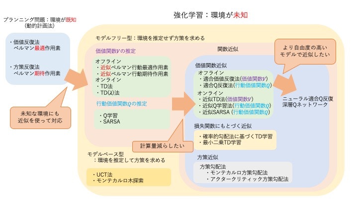
Planning Problems

Sequential decision-making problems where the environment dynamics (state transition probabilities and reward functions) are known.

• Value Iteration Directly computes the optimal value function by repeatedly applying the Bellman optimality operator.

  \[ (B_{\*}v)(s) = \max_a \{g(s,a) + \gamma \sum_{s'} p_T(s'|s,a)v(s')\} \] \[ V^{\*} = \lim_{k \to \infty} (B_{*}^{k}V)(s) \]

• Policy Iteration Iterates between two steps – “policy evaluation” and “policy improvement” – to find the optimal policy.

  1. Policy Evaluation: Computes the value function \(V^\pi\) under the current policy \(\pi\) using the Bellman expectation operator. \( (B_{\pi}v)(s) = \sum_a \pi(a|s) (g(s,a) + \gamma \sum_{s'} p_T(s'|s,a)v(s')) \) \( V^{\pi} = \lim_{k \to \infty} (B_{\pi}^{k}V)(s) \)
  2. Policy Improvement: Greedily determines a better policy using the computed value function \(V^\pi\) . \( \pi(s) = \arg\max_a \{g(s,a) + \gamma \sum_{s'} p_T(s'|s,a)V^\pi(s')\} \)

Reinforcement Learning

The planning problems above assumed that the transition probabilities \(p_T(s'|s,a)\) and reward function \(g(s,a)\) – the environment model – are known, and used dynamic programming (repeated application of a Bellman operator) to find the optimal policy. In most real-world problems (robot control, games, and so on), however, this environment model is unknown. Reinforcement learning addresses sequential decision-making problems where the environment dynamics are unknown: the agent learns value functions and policies directly from experience (sequences of states, actions, and rewards) gathered by actually interacting with the environment, without ever going through a model.

Without a model, how can the agent estimate value at all? Two broad families of answers exist.

Monte Carlo and TD Learning: Two Ways to Estimate Value Without a Model

Going back to the definition of the state-value function \(V^\pi(s) = \mathbb{E}_\pi[G_t \mid S_t=s]\) (where \(G_t = r_t + \gamma r_{t+1} + \gamma^2 r_{t+2} + \dots\) is the discounted return from time \(t\) onward), the most naive way to estimate it is to run an episode to completion and use the return \(G_t\) that was actually observed as the value estimate. This is the Monte Carlo (MC) method.

Because \(G_t\) is computed purely from rewards actually observed from the environment, no estimate other than the true value function ever enters the update – MC is unbiased. But it has two drawbacks. First, computing \(G_t\) requires waiting until the episode terminates, so for long episodes (or continuing tasks that never terminate) the update frequency becomes extremely low. Second, \(G_t\) is a realization of a random variable that folds in every future reward and action choice, so it tends to have high variance.

On the other hand, writing the Bellman expectation equation (see the Planning Problems section) for the state-value function gives

This identity holds exactly if we know the true \(V^\pi\) , but the estimate \(\hat V\) we have mid-training generally does not satisfy it. TD learning (Temporal-Difference learning) – specifically TD(0) – replaces the expectation on the right-hand side of Eq. (1) with a single-sample realization \(r_t + \gamma \hat V(s_{t+1})\) , treats it as a “provisional target” (the TD target), and corrects \(\hat V(s_t)\) by the gap between the two,

The TD error \(\delta_t\) is nothing but the residual of the Bellman expectation equation (1) evaluated at the current estimate \(\hat V\) . If \(\delta_t\) were identically zero at every state, \(\hat V\) would satisfy Eq. (1) – i.e., it would have converged to the fixed point \(V^\pi\) of the Bellman expectation operator. The TD target \(r_t + \gamma \hat V(s_{t+1})\) is also a bootstrap (self-reference): it estimates future value using \(\hat V(s_{t+1})\) , which may itself still be inaccurate mid-training. This is the essential difference from Monte Carlo.

Bootstrapping lets TD learning update after every single step (without waiting for episode termination) even though the true \(V^\pi\) is unknown, and because each update uses only one step’s worth of reward, its variance is lower than MC’s. In exchange, while \(\hat V(s_{t+1})\) is still inaccurate early in training, the TD target carries a systematic bias. In short, MC and TD trade off “unbiased but high-variance, low-frequency updates” against “biased but low-variance, high-frequency (online) updates.” We verify this difference numerically in the Cliff Walking experiment below.

Value-Based Methods

These methods estimate a value function (state-value function V or action-value function Q) and implicitly derive a policy from it. Applying the TD(0) update derived above to the action-value function \(Q(s,a)\) instead of the state-value function gives Q-Learning and SARSA.

• Q-Learning The action-value function also satisfies a Bellman optimality equation:

  \[ Q^*(s,a) = \mathbb{E}\big[r_t + \gamma \max_{a'} Q^*(s_{t+1}, a') \mid s_t=s, a_t=a\big] \tag{2} \]

  Replacing the expectation on the right-hand side of Eq. (2) with the single-sample realization \(r_t + \gamma \max_{a'} \hat Q(s_{t+1},a')\) and using it as the TD target to correct \(\hat Q(s_t,a_t)\) gives Q-Learning.

  \[ \delta_t = r_t + \gamma \max_{a'} \hat{Q}(s_{t+1}, a') - \hat{Q}(s_t, a_t) \] \[ \hat{Q}(s_t, a_t) \leftarrow \hat{Q}(s_t, a_t) + \alpha_t \delta_t \]

  Equation (2) is an identity about the optimal value function \(Q^*\) itself, not about any particular policy, and the \(\max_{a'}\) on the right-hand side does not depend at all on which action the agent actually took next. This means Q-Learning’s TD target can be computed from just the transition \((s_t,a_t,r_t,s_{t+1})\) , regardless of which behavior policy (e.g. an \(\varepsilon\) -greedy exploration policy) generated it. This is why Q-Learning is called off-policy: it converges to \(Q^*\) itself, independent of the exploration policy (given that every state-action pair is visited sufficiently often and \(\alpha_t\) decays appropriately).

• SARSA Meanwhile, fixing a policy \(\pi\) , the action-value function \(Q^\pi\) under it satisfies a Bellman expectation equation:

  \[ Q^\pi(s,a) = \mathbb{E}_\pi\big[r_t + \gamma Q^\pi(s_{t+1}, a_{t+1}) \mid s_t=s, a_t=a\big] \tag{3} \]

  Here \(a_{t+1}\) on the right-hand side is the action actually chosen according to policy \(\pi\) (e.g. \(\varepsilon\) -greedy). Replacing the expectation with this single-sample realization \(r_t + \gamma \hat Q(s_{t+1},a_{t+1})\) gives

  \[ \delta_t = r_t + \gamma \hat{Q}(s_{t+1}, a_{t+1}) - \hat{Q}(s_t, a_t) \] \[ \hat{Q}(s_t, a_t) \leftarrow \hat{Q}(s_t, a_t) + \alpha_t \delta_t \]

  This is SARSA (State-Action-Reward-State-Action). Since Eq. (3) is an identity about the policy \(\pi\) itself, what SARSA learns is the action-value function of “whatever policy is currently being executed” – which is why it is called on-policy.

The Q-Learning and SARSA update rules differ in exactly one place – \(\max_{a'}\hat Q(s_{t+1},a')\) versus \(\hat Q(s_{t+1},a_{t+1})\) – but under an exploratory policy (\(\varepsilon\) -greedy with \(\varepsilon>0\) ) they can converge to different fixed points. Q-Learning converges to the optimal value function \(Q^*\) (the value of the purely greedy policy with no exploration at all) regardless of the exploration policy, whereas SARSA converges to \(Q^{\pi_\varepsilon}\) , the value function of the policy \(\pi_\varepsilon\) that includes the exploration itself. In other words, the “good actions” SARSA learns already price in the risk of occasionally failing badly due to \(\varepsilon\) -greedy’s random exploration. We verify this difference numerically on the famous Cliff Walking problem.

Verifying the Difference Between Q-Learning and SARSA: Cliff Walking

Setup: a 4-row by 12-column grid. The agent starts at the bottom-left \((3,0)\) and must reach the goal at the bottom-right \((3,11)\) . The bottom row from \((3,1)\) to \((3,10)\) is a “cliff”: stepping into it yields a reward of \(-100\) and sends the agent back to the start (the episode does not terminate). Every other transition yields a reward of \(-1\) per step. We used a discount factor \(\gamma=1\) , learning rate \(\alpha=0.5\) , and a fixed (non-decaying) \(\varepsilon\) -greedy exploration rate of \(\varepsilon=0.1\) .

import numpy as np

n_rows, n_cols = 4, 12
start, goal = (3, 0), (3, 11)
cliff = [(3, c) for c in range(1, 11)]

def step(state, action):  # 0:up 1:right 2:down 3:left
    r, c = state
    if action == 0: r = max(r - 1, 0)
    elif action == 1: c = min(c + 1, n_cols - 1)
    elif action == 2: r = min(r + 1, n_rows - 1)
    elif action == 3: c = max(c - 1, 0)
    ns = (r, c)
    if ns in cliff:
        return start, -100, False       # fall off the cliff, back to start (episode continues)
    if ns == goal:
        return ns, -1, True             # reaching the goal ends the episode
    return ns, -1, False

# Q-Learning: bootstraps off max_a' Q(s',a') at the next state (off-policy)
Q[s][a] += alpha * (r + gamma * Q[ns].max() - Q[s][a])

# SARSA: bootstraps off Q(s',a') for the action a' actually chosen next (on-policy)
Q[s][a] += alpha * (r + gamma * Q[ns][na] - Q[s][a])

Training for 500 episodes and averaging over 100 independent runs gave the following results.

• Greedy policy after training (tested with \(\varepsilon=0\) ): Q-Learning learned the 13-step, reward \(-13\) shortest path – walking right along the row directly above the cliff (row 2) for 11 columns before dropping down to the goal. SARSA learned a 17-step, reward \(-17\) detour that climbs all the way to the top row (row 0) before crossing, staying well away from the cliff.
• Online average reward during training (with \(\varepsilon=0.1\) exploration active): over the second half of training (episodes 401-500), the average was -49.89 for Q-Learning versus -26.09 for SARSA (over the first 100 episodes, the averages were -80.52 and -71.45, respectively).

Even though the greedy policy Q-Learning converges to is truly optimal (the shortest path), its measured online performance during training was substantially worse than SARSA’s. The reason is exactly the difference between Eq. (2) and Eq. (3). Because Q-Learning’s TD target always uses \(\max_{a'}\) , the “aggressive” path hugging the cliff edge gets a high value estimate – but the data is actually collected by the \(\varepsilon\) -greedy behavior policy, which takes a random action with probability \(\varepsilon\) , and while walking next to the cliff this occasionally sends the agent tumbling in for a \(-100\) . SARSA’s TD target, on the other hand, uses the action \(a_{t+1}\) that is actually chosen next (i.e. it includes the \(\varepsilon\) -greedy randomness), so the “fall risk” of standing next to the cliff is directly reflected in the Q-values, making the safer, cliff-avoiding path the more highly valued one. This shows up clearly in the learning curves from the actual exploring environment.

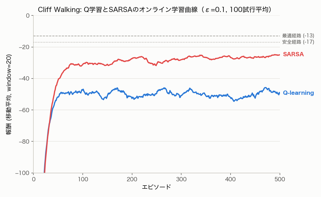
As the learning curves above show, SARSA consistently achieves a higher (less negative) online reward than Q-Learning. Both improve rapidly early on and then fluctuate with the exploration noise, but SARSA’s converged level stabilizes roughly 20-25 points above Q-Learning’s.

We further implemented Monte Carlo control (first-visit MC control, with a constant step size \(\alpha=0.5\) and each episode capped at 300 steps) on the same environment for comparison.

G = 0
visited = set()
for s, a, r in reversed(episode):
    G = r + gamma * G
    if (s, a) not in visited:
        visited.add((s, a))
        Q[s][a] += alpha * (G - Q[s][a])

Averaged over 100 runs of 500 episodes, MC control’s average reward was -1051.11 over the first 100 episodes and improved to only -537.56 by the last 100 – nearly two orders of magnitude worse than either Q-Learning or SARSA. Testing the resulting greedy policy, it failed to reach the goal within a 200-step cap and instead got stuck oscillating in the top-left corner state – an essentially unlearned policy.

This is exactly the weakness of Monte Carlo methods discussed earlier, made concrete. MC cannot update any state-action pair until an episode finishes, and in this environment, under the near-random policy of early training, episodes tend to become extremely long (repeatedly bounced back to the start by the cliff) – so learning only ever sees incomplete episodes truncated at 300 steps, and can fill in the values of \(48\) states \(\times\, 4\) actions with at most a few dozen updates per episode. TD-based Q-Learning and SARSA, by contrast, update from every single transition at every step, so they accumulate far more updates over the same 500 episodes. This experiment shows that bootstrapping is not merely a theoretical nicety – it produces a real, practical difference in learning speed whenever episodes are long or their length is uncertain.

Policy-Based Methods

These methods directly model and optimize the policy \(\pi_\theta\) with parameters \(\theta\) , without going through a value function.

• Policy Gradient Methods Compute the gradient \(\nabla_\theta J(\theta)\) to maximize a performance measure \(J(\theta)\) , and update the policy parameters \(\theta\) . \( \theta_{t+1} = \theta_t + \alpha \nabla_\theta J(\theta_t) \)

Deriving the Policy Gradient Theorem

Suppose we want to update the policy parameters \(\theta\) to maximize the performance measure

where \(\tau=(s_0,a_0,r_0,s_1,a_1,r_1,\dots)\) is a trajectory generated under policy \(\pi_\theta\) , and \(p_\theta(\tau)\) is its probability of occurring.

Differentiating \(J(\theta)\) directly with respect to \(\theta\) gives

but \(\nabla_\theta p_\theta(\tau)\) is not itself an expectation, so this cannot be approximated by sampling. Using the log-derivative trick – the identity \(\nabla_\theta p_\theta(\tau) = p_\theta(\tau) \nabla_\theta \log p_\theta(\tau)\) , obtained simply by multiplying both sides of \(\nabla_\theta \log p_\theta(\tau) = \nabla_\theta p_\theta(\tau)/p_\theta(\tau)\) by \(p_\theta(\tau)\) – we get

which can now be estimated simply by sampling \(\tau \sim p_\theta\) and averaging. All that remains is to work out \(\log p_\theta(\tau)\) explicitly. By the Markov property and the independence of the action choice at each step, the trajectory probability factorizes as

so that

Here, neither the initial state distribution \(p(s_0)\) nor the environment’s transition probability \(p_T(s_{t+1}|s_t,a_t)\) depends on the policy parameters \(\theta\) , so both vanish upon differentiating with respect to \(\theta\) :

This is a decisive property for model-free reinforcement learning: it means the policy gradient \(\nabla_\theta J(\theta)\) can be computed without ever knowing the environment’s transition probabilities \(p_T\) – they simply never appear in the formula. Putting it together,

Next, using causality – the fact that the action \(a_t\) at time \(t\) cannot influence rewards \(r_0,\dots,r_{t-1}\) that occurred before it – one can show that replacing \(R(\tau)\) inside the sum with the discounted return from time \(t\) onward, \(G_t = \sum_{k=t}^T \gamma^{k-t} r_k\) , leaves the expectation unchanged. (The reward terms before time \(t\) are independent of \(\nabla_\theta \log \pi_\theta(a_t|s_t)\) and can be pulled outside the expectation, where their contribution vanishes because the action probabilities sum to one.) Using the definition of the conditional expectation \(\mathbb{E}[G_t\mid s_t,a_t]=Q^{\pi_\theta}(s_t,a_t)\) , we finally obtain the policy gradient theorem:

(Written as an expectation over the stationary state distribution \(d^{\pi_\theta}(s)\) , this becomes \(\nabla_\theta J(\theta) = \sum_s d^{\pi_\theta}(s)\sum_a \pi_\theta(a|s)\nabla_\theta \log \pi_\theta(a|s)Q^{\pi_\theta}(s,a)\) .) When \(Q^{\pi_\theta}\) is unknown and is replaced by the actually observed Monte Carlo return \(G_t\) , the resulting algorithm is REINFORCE.

Putting REINFORCE to the Test: A Comparison with Q-Learning

The derivation above is complete on paper, but it does not tell us how policy-gradient methods actually behave compared to value-based methods in practice – in particular, whether the “TD bootstrapping vs. Monte Carlo” trade-off discussed in the previous section shows up in the same form when optimizing a policy directly. To check this, we train Q-Learning (value-based) and REINFORCE (policy-based) on exactly the same environment and compare them directly.

Setup: a 5-row by 5-column grid. The agent starts at the top-left \((0,0)\) and must reach the goal at the bottom-right \((4,4)\) . There is no cliff-like trap; every step yields a reward of \(-1\) , and the episode ends upon reaching the goal (the final \(-1\) is included). Discount factor \(\gamma=1\) . The optimal path length is the Manhattan distance, \(8\) steps, giving an optimal return of \(-8\) .

REINFORCE’s policy is a tabular softmax with parameters \(\theta_{s,a}\) per state, \(\pi_\theta(a|s) \propto \exp(\theta_{s,a})\) . There is an important implementation detail here. Using the raw softmax directly, the policy is strongly attracted early in training toward looping trajectories that are “not catastrophic like falling off a cliff, but never reach the goal either,” and \(\theta\) saturates so quickly that exploration tends to stall (we verified this directly: removing the exploration floor clearly worsened the goal-reaching rate, though the exact magnitude of the degradation is sensitive to implementation details — the learning-rate schedule, how theta is initialized, which RNG is used — so we won’t commit to a single precise figure here). To prevent this, we mix in the same \(\varepsilon=0.1\) exploration floor used for Q-Learning’s \(\varepsilon\) -greedy action selection, applied here to the policy’s own action selection as well.

def mixed_policy(theta_s, eps=0.1):
    p_soft = softmax(theta_s)
    return (1 - eps) * p_soft + eps / n_actions, p_soft

# Q-Learning (value-based, eps-greedy action selection, off-policy): same TD(0) update as before
Q[s][a] += alpha * (r + gamma * Q[ns].max() - Q[s][a])

# REINFORCE (policy-based): compute d/dtheta_k log p_mix(a|s) via the chain rule, then ascend
p_mix, p_soft = mixed_policy(theta[s])
grad = -p_soft * p_soft[a]
grad[a] += p_soft[a]
grad *= (1 - eps) / p_mix[a]
theta[s] += alpha * advantage * grad  # advantage = G_t (no baseline) or G_t - V[s] (with baseline)

We used a learning rate of \(\alpha=0.5\) for Q-Learning and \(\alpha=0.05\) for REINFORCE (with \(\alpha_V=0.1\) when using \(\hat V\) ), training for 500 episodes and averaging over 100 independent runs with seeds 2000 through 2099 (capped at 100 steps per episode).

• Q-Learning: average reward improved from -20.84 over the first 50 episodes to -8.83 over the last 50 (episodes 451-500); the resulting greedy policy reached the goal in 99 out of 100 runs, with mean return -8.92 (close to the optimum of \(-8\) ).
• REINFORCE (no baseline): improved only from -69.94 to -25.12; the greedy policy’s goal-reaching rate was 79/100, with mean return -27.86.
• REINFORCE (with a Monte Carlo state-value estimate as baseline): improved from -52.55 to -15.22; the greedy policy’s goal-reaching rate was 94/100, with mean return -13.80.

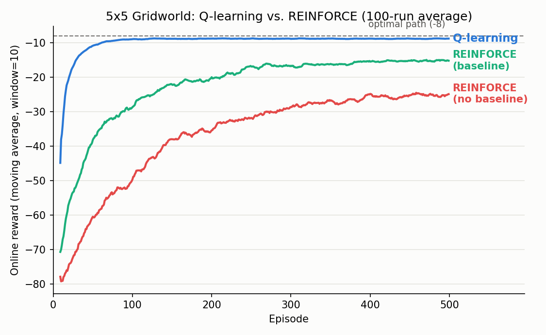
Over the same 500 episodes, Q-Learning reaches near-optimal performance within roughly 100 episodes, while both REINFORCE variants lag far behind. This shows that the “TD learning bootstraps and updates every single step, while Monte Carlo must wait for the episode to end and has higher variance” trade-off we confirmed in the Cliff Walking section applies not only to estimating a state-value function, but equally to optimizing the policy itself. Q-Learning updates \(Q\) from the TD error after every single transition, and that information propagates to other states via bootstrapping, whereas REINFORCE’s gradient can only be weighted by the whole-episode return \(G_t\) (a high-variance random variable), requiring many episodes for the noise to average out before the policy can move reliably in the right direction. The gap between the baseline and no-baseline variants (goal-reaching rate 79% -> 94%, mean return \(-27.86 \to -13.80\) ) is exactly the variance-reduction effect we derive theoretically in the next section, showing up in practice.

Actor-Critic Methods

These methods combine value-based and policy-based approaches.

• Actor: Updates the policy \(\pi_\theta\) (selects actions)
• Critic: Learns a value function and evaluates the actions chosen by the actor

Both the actor and critic are updated using the TD error \(\delta_t\) .

Variance Reduction with a Baseline

The REINFORCE gradient \(\nabla_\theta \log \pi_\theta(a_t|s_t) G_t\) is an unbiased estimator, but \(G_t\) is a sum over a stochastic sequence of future rewards, so its variance is large and can make learning unstable. Subtracting any function \(b(s)\) that depends only on the state \(s\) and not on the action \(a\) – a baseline – from the gradient leaves the expectation unchanged, as the following identity shows:

(using the identity \(\sum_a \pi_\theta(a|s)=1\) , which holds for every \(\theta\) ). Hence

remains unbiased for any choice of \(b(s)\) . Choosing \(b(s) = V^{\pi_\theta}(s)\) in particular turns the term in parentheses into the advantage function, \(A^{\pi_\theta}(s,a) = Q^{\pi_\theta}(s,a) - V^{\pi_\theta}(s)\) . \(A^{\pi_\theta}(s,a)\) measures “how much better (or worse) taking action \(a\) is compared to the average value \(V(s)\) of state \(s\) ,” and its range (and hence variance) is smaller than \(Q\) alone, which reduces the variance of the gradient estimate.

Unbiasedness is proven above, but it is worth checking numerically how much the variance actually drops. Using the same 5x5 gridworld from the previous section, we rolled out 3000 episodes from the initial policy (uniform, \(\theta=0\) ; seed 7), and for each episode computed the norm of the policy-gradient estimate \(\sum_t \nabla_\theta \log \pi_\theta(a_t|s_t)\,G_t\) , as well as the norm with the baseline (a Monte Carlo estimate \(\hat V\) of the posterior mean return observed from that state) subtracted: \(\sum_t \nabla_\theta \log \pi_\theta(a_t|s_t)\,(G_t - \hat V(s_t))\) , over all 3000 samples. The mean gradient norm dropped from \(290.5\) to \(162.4\) , and its variance dropped from \(28471.1\) to \(3725.2\) – a reduction of roughly 7.6x. The estimate’s spread shrinks dramatically while its average direction (unbiasedness) is preserved. This is exactly what underlies why REINFORCE-with-baseline learned the goal-reaching path faster and more reliably than REINFORCE-without-baseline in the previous section (the variance of the online reward itself, compared late in training, also dropped by about 2.3x, from \(1016.8\) to \(436.2\) ).

Actor-Critic methods estimate this advantage function by separately learning a value function. Using the Bellman relation

the conditional expectation of the TD error works out to

so the TD error \(\delta_t\) – a quantity the critic can compute from a single step of observation – is exactly an unbiased single-sample estimator of the advantage function. This is why the actor’s (policy’s) update can use the TD error \(\delta_t\) computed by the critic directly, in place of \(Q\) itself.

• Critic Update (Value Function Learning) \( \delta_t = r_t + \gamma \hat{V}_w(s_{t+1}) - \hat{V}_w(s_t) \) \( w_{t+1} = w_t + \alpha_w \delta_t \nabla_w \hat{V}_w(s_t) \)
• Actor Update (Policy Learning): as derived above, \(\delta_t\) is an unbiased estimator of the advantage function, so it is used directly as the weight in the policy gradient. \( \theta_{t+1} = \theta_t + \alpha_\theta \delta_t \nabla_\theta \log \pi_\theta(a_t|s_t) \)

A Further Development: Baselines Without a Critic – GRPO (2024)

So far we have seen two concrete choices of the baseline \(b(s)\) : a Monte Carlo estimate \(\hat V(s)\) (previous section), and a critic \(\hat V_w(s)\) learned by TD bootstrapping (Actor-Critic). But as shown just before Eq. (4), unbiasedness only requires \(b(s)\) to be “some function of the state \(s\) that does not depend on the action \(a\) ” – so many other choices are possible.

GRPO (Group Relative Policy Optimization), proposed in 2024 to improve the mathematical reasoning ability of large language models, exploits exactly this freedom to dispense with the critic altogether. For the same state (prompt) \(s\) , it independently samples \(G\) trajectories (responses) from the policy, and estimates the advantage directly from the relative standing of the resulting rewards \(r_1,\dots,r_G\) within that group:

Here \(\mathrm{mean}(r_1,\dots,r_G)\) is computed purely from the \(G\) samples drawn from the same state \(s\) , and does not depend on any individual action \(a_i\) – so it is precisely an instance of the “any \(b(s)\) that does not depend on the action” result we proved above. In other words, GRPO replaces a learned critic with an empirically estimated baseline obtained by sampling the same state multiple times. Because this eliminates the need to train a separate value-function network (the critic) at all, it is a substantial saving in compute and memory when the policy itself is a massive language model (Shao et al., “DeepSeekMath: Pushing the Limits of Mathematical Reasoning in Open Language Models,” arXiv:2402.03300 , 2024).

Dropping the critic is not without cost, however. de Oliveira et al. (2025) systematically evaluated GRPO on classical single-task reinforcement learning environments much like the ones in this article (discrete and continuous control tasks), and found that methods with a learned critic (such as PPO) consistently outperform critic-free methods, except in short-horizon tasks like CartPole (“Learning Without Critics? Revisiting GRPO in Classical Reinforcement Learning Environments,” arXiv:2511.03527 , 2025). This is consistent with our own experimental results in this article: TD-based bootstrapping methods had an overwhelming advantage on Cliff Walking, where episodes tend to be long (and so benefit greatly from bootstrapping), whereas on the short-horizon 5x5 gridworld, a simple Monte Carlo baseline alone already produced a large improvement. It is striking that the same intuition – that a critic (bootstrapping) becomes essential precisely for long-horizon problems – is being rediscovered in the 2020s in the context of reinforcement learning for LLMs.

Function Approximation

When the state space is large or continuous, value functions and policies are approximated using parameterized functions (such as linear functions or neural networks) with parameters \(w\) or \(\theta\) , instead of tabular representations.

• Value Function Approximation Combines function approximation with update rules such as TD learning and Q-Learning. For example, in approximate Q-Learning, the weights \(w\) are updated as follows:

  \[ \delta_t = r_t + \gamma \max_{a'} \hat{Q}_w(s_{t+1}, a') - \hat{Q}_w(s_t, a_t) \] \[ w_{t+1} = w_t + \alpha_t \delta_t \nabla_w \hat{Q}_w(s_t, a_t) \]

  Deep Q-Network (DQN) uses a neural network to approximate the action-value function, but naively applying the update rule above to a neural network is known to make training unstable or even divergent. There are two main causes.

  1. Correlated samples: the sequence of transitions \((s_t,a_t,r_t,s_{t+1})\) the agent generates is strongly correlated in time, violating the independent-and-identically-distributed (i.i.d.) sample assumption that stochastic gradient descent relies on. Training on a run of similar consecutive states causes the network to overfit to that local pattern and destroy its value estimates for other states (catastrophic forgetting).
  2. A moving target: the TD target in the update rule, \(r_t + \gamma \max_{a'} \hat Q_w(s_{t+1},a')\) , is computed using the very parameters \(w\) that are being updated right now. Every time \(w\) takes a step, the target itself shifts – so, viewed as a regression problem, the target is non-stationary and keeps moving, which makes the value estimate prone to diverging. In tabular Q-Learning, updating one state’s Q-value leaves every other state’s Q-value untouched; but with a function approximator like a neural network, parameters are shared across states, so an update at one state can (unintentionally) shift the estimates at many other states as well – making this problem considerably worse.

  DQN addresses these two problems with two corresponding techniques.

  • Experience Replay: transitions \((s_t,a_t,r_t,s_{t+1})\) are stored in a large buffer, and training samples random minibatches from it instead of using consecutive transitions directly. Mixing together transitions that are not adjacent in time approximates an i.i.d. sample set and mitigates the correlation problem. It also improves sample efficiency by letting past experience be reused repeatedly.
  • Target Network: a separate copy of the parameters, \(w^-\) , is kept purely for computing targets, distinct from the online parameters \(w\) that are updated every step by gradient descent. \(w^-\) is only synced to the current value of \(w\) at fixed intervals (e.g. every few thousand steps). Because the TD target is always computed with this frozen \(w^-\) (i.e. \(r_t + \gamma \max_{a'} \hat Q_{w^-}(s_{t+1},a')\) ), the training target is temporarily frozen, which mitigates the moving-target problem.

• Policy Function Approximation Directly approximates the policy using function approximation in policy gradient methods and actor-critic methods.

Related Articles

• Reinforcement Learning Basics: Markov Decision Processes and the Bellman Equations - Formalizing MDPs, proving the Bellman equations, and implementing value/policy iteration
• Model-Free Reinforcement Learning - The exploration-exploitation trade-off and TD(\(\lambda\) )
• Policy Gradient Methods - A closer look at the policy gradient theorem
• Advantage Actor-Critic (A2C) - Actor-Critic with the advantage function
• Key Algorithms in Deep Reinforcement Learning - Algorithms building on DQN

References

• Tetsuro Morimura, “ MLP Machine Learning Professional Series: Reinforcement Learning ”