Fundamentals of Filtering Methods in Signal Processing

What is Filtering?

Filtering is a technique for removing noise components from observed time-series data and extracting the underlying signal.

State-Space Model

In filtering, we estimate the internal state \(x_t\) , which cannot be directly observed, from observations \(z_t\) . The system behavior is represented by two models:

• Process Model (System Model): Describes how the state \(x_t\) evolves over time.

• Observation Model: Describes how observations \(z_t\) are generated from the state \(x_t\) .

Here, \(u_t\) is the control input, and \(q_t\) and \(r_t\) are the process noise and observation noise, respectively, which are generally assumed to follow zero-mean Gaussian distributions.

\(Q\) and \(R\) are the noise covariance matrices. The Kalman filter described below is exactly optimal only when both \(f\) and \(h\) are linear maps (\(f(x)=Ax\) , \(h(x)=Hx\) ) and the noise is Gaussian. Otherwise, approximate methods such as the EKF, UKF, or particle filter are needed.

Kalman Filter (KF)

Overview

The KF is an optimal filter that accurately estimates the mean and covariance of the state under the assumptions that the system is linear and that the noise follows a Gaussian distribution. It sequentially estimates the state by repeating two steps: “prediction” and “update (filtering).”

Algorithm

The probability distribution of state \(x\) is represented by its mean \(\mu\) and covariance \(\Sigma\) .

1. Prediction Step: Predicts the current state from the previous state estimate.

• Prior state estimate: Predicts the current state \(\hat{\mu}_t\) from the previous state \(\mu_{t-1}\) .

• Prior error covariance matrix: Computes the prediction uncertainty \(\hat{\Sigma}_t\) .

2. Update Step: Corrects the prediction with the observation \(z_t\) to obtain a more accurate current state estimate.

• Kalman gain: A coefficient that determines how much to weight the prediction versus the observation.

• Posterior state estimate: Corrects the predicted value \(\hat{\mu}_t\) with the observation \(z_t\) .

• Posterior error covariance matrix: Computes the updated uncertainty \(\Sigma_t\) .

Derivation: Why the Kalman Gain Formula Is Optimal

Equation (5) may look like it was handed down from nowhere, but it is actually the solution to an optimization problem: “combine two unbiased estimates – the prediction and the observation – linearly so as to minimize the posterior variance.” The full multivariate derivation and implementation are covered in Kalman Filter Theory and Python Implementation ; here we show the essence using the scalar case (\(H=1\) ).

The predicted state \(\hat{\mu}_t\) (error variance \(\hat{\sigma}_t^2\) ) and the observation \(z_t\) (observation noise variance \(R\) ) are both independent, unbiased estimates of the true state \(x_t\) . Consider a linear combination of the two with weight \(K\) :

Since \(\mathbb{E}[\hat{\mu}_t]=\mathbb{E}[z_t]=x_t\) , \(\mu_t\) is unbiased for any choice of \(K\) . Because the two estimates are independent, the variance is

To find the \(K\) that minimizes this variance, differentiate with respect to \(K\) and set the result to zero:

Solving for \(K\) gives

which is exactly equation (5) with \(H=1\) . In other words, the Kalman gain is a precision-weighted average (weighted by the inverse of variance): it favors the observation when the prediction is uncertain (\(\hat{\sigma}_t^2\) large), and favors the prediction when the observation is noisy (\(R\) large) – all derived purely from minimizing variance. Substituting equation (9) back into equation (8) gives

which matches equation (7) evaluated at \(H=1\) . In the multivariate case, the same result follows from minimizing the trace of the posterior covariance \(\Sigma_t\) (the sum of the variances of each component) with respect to \(K_t\) – this is the Best Linear Unbiased Estimator (BLUE) property from the Gauss-Markov theorem. When the noise is Gaussian, the posterior itself is Gaussian, so this linear estimator is not just optimal among linear estimators but is the minimum-variance estimator among all estimators, linear or not (it coincides with both the MAP and MMSE estimator).

Numerical Experiment: Estimating a 1D Random Walk

To confirm that the derived Kalman filter actually reduces noise, we test it on the simplest possible 1D model. The true state follows a random walk \(x_t = x_{t-1} + q_t\) (\(q_t \sim \mathcal{N}(0, Q)\) , \(Q=0.25\) ), and the observation is \(z_t = x_t + r_t\) (\(r_t \sim \mathcal{N}(0, R)\) , \(R=4.0\) ) (a scalar Kalman filter with \(A=H=1\) ).

import numpy as np

np.random.seed(0)

T = 50
Q = 0.25  # process noise variance
R = 4.0  # observation noise variance

x_true = np.zeros(T + 1)
z = np.zeros(T + 1)
for t in range(1, T + 1):
    x_true[t] = x_true[t - 1] + np.random.normal(0, np.sqrt(Q))
z[1:] = x_true[1:] + np.random.normal(0, np.sqrt(R), size=T)

# --- Scalar Kalman filter (A=H=1) ---
mu, sigma2 = 0.0, 1.0  # initial state estimate and variance
mu_hist, sigma2_hist, K_hist = [mu], [sigma2], []

for t in range(1, T + 1):
    mu_pred = mu  # prediction step (Eq. 3, A=1)
    sigma2_pred = sigma2 + Q  # prediction step (Eq. 4)

    K = sigma2_pred / (sigma2_pred + R)  # Kalman gain (Eq. 9)
    mu = mu_pred + K * (z[t] - mu_pred)  # update step (Eq. 6)
    sigma2 = (1 - K) * sigma2_pred  # update step (Eq. 7)

    mu_hist.append(mu)
    sigma2_hist.append(sigma2)
    K_hist.append(K)

mu_hist, sigma2_hist = np.array(mu_hist), np.array(sigma2_hist)
rmse_obs = np.sqrt(np.mean((z[1:] - x_true[1:]) ** 2))
rmse_kf = np.sqrt(np.mean((mu_hist[1:] - x_true[1:]) ** 2))

print(f"K_1 = {K_hist[0]:.4f}, K_50 = {K_hist[-1]:.4f}")
print(f"RMSE(observation) = {rmse_obs:.4f}, RMSE(KF estimate) = {rmse_kf:.4f}")

Running this yields:

K_1 = 0.2381, K_50 = 0.2207
RMSE(observation) = 1.7346, RMSE(KF estimate) = 1.4041

As predicted by equation (9), the initial variance \(\hat{\sigma}_1^2 = 1.0 + Q = 1.25\) gives \(K_1 = 1.25/(1.25+4.0) = 0.2381\) , matching the measured value exactly. Even though the observation noise standard deviation (\(\sqrt{R}=2.0\) ) is large, the Kalman filter reduces the RMSE from 1.735 (raw observations) to 1.404 (KF estimate) – roughly a 19% reduction in error. The figure below shows the true state, observations, and KF estimate (with a \(\pm 2\sigma\) band).

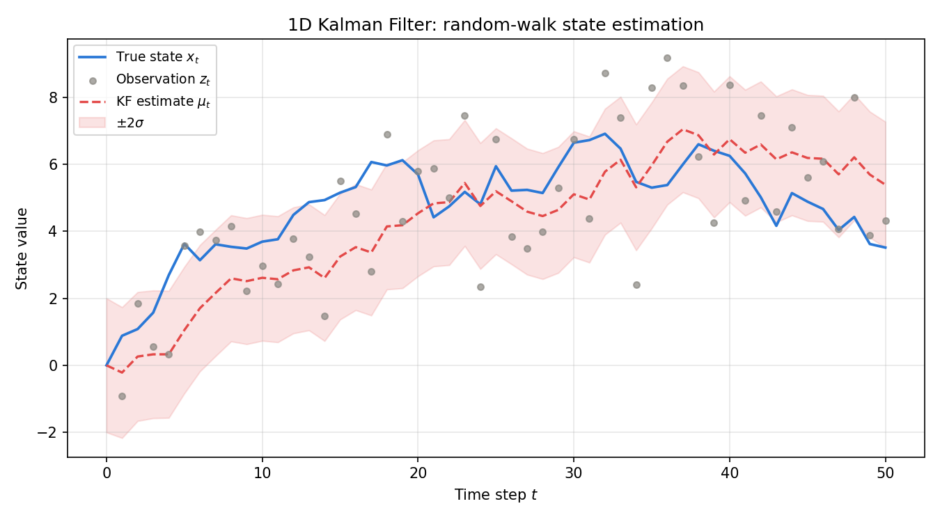
The estimate (red dashed line) tracks the true state (blue line) more smoothly than the raw observations (gray dots), and the \(\pm 2\sigma\) band covers nearly all of the true trajectory. For a more practical example using a 1D constant-velocity model, see Kalman Filter Theory and Python Implementation .

Extended Kalman Filter (EKF)

Overview

The EKF extends the KF to handle nonlinear systems. It applies the KF framework by linearizing the nonlinear functions around the current state estimate using a first-order Taylor expansion.

Method

The process model \(f\) and observation model \(h\) are linearized using Jacobian matrices (partial derivatives).

These \(F_t\) and \(H_t\) are used in place of \(A\) and \(H\) in the linear Kalman filter equations, though the prediction step uses the nonlinear functions directly.

• Limitation: For highly nonlinear systems, the linearization error becomes large, potentially degrading estimation accuracy or causing divergence.

Derivation: When Is First-Order Linearization Valid?

To see why the EKF’s “linearization via the Jacobian” is justified, consider the Taylor expansion of the observation model \(h\) around the current estimate \(\hat{\mu}_t\) :

where \(\nabla^2 h\) is the Hessian matrix (second derivatives) of \(h\) . The EKF keeps only the first term (constant) and the second term (the linear Jacobian term) of equation (10), and discards the curvature term entirely. This approximation is valid when the state error covariance \(\hat{\Sigma}_t\) is small enough, and the curvature \(\nabla^2 h\) is approximately constant near the estimate. Indeed, taking the expectation over the distribution of \(x\) gives

so the size of the second-order term the EKF ignores is governed by the trace of the product of the curvature \(\nabla^2 h\) and the covariance \(\hat{\Sigma}_t\) . Consequently, when the covariance is large or the nonlinearity (curvature) is strong, this neglected term becomes non-negligible, and the EKF estimate develops a systematic bias, underestimates its own covariance, and can diverge. Concrete examples of this linearization error and divergence, along with recent extensions that use neural networks to learn the curvature correction from data, are covered in detail in Extended Kalman Filter Theory and Python Implementation .

Unscented Kalman Filter (UKF)

Overview

Like the EKF, the UKF handles nonlinear systems, but instead of directly linearizing the functions, it uses the Unscented Transform to propagate the probability distribution of the state.

Method

A small set of representative points (sigma points) that capture the current state distribution are sampled and passed through the nonlinear function. The mean and covariance are then recomputed from the transformed points using weighted averages, achieving higher accuracy than the EKF.

• Advantage: No Jacobian computation is required, and it is more robust than the EKF for highly nonlinear systems.

Intuition: Why Is the UKF Accurate to Second Order?

Where the EKF captures only the first-order Taylor term, the UKF captures the second-order term as well. To see why, consider the scalar (single-variable) case. For a state \(x \sim \mathcal{N}(\mu, \sigma^2)\) passed through a nonlinear function \(g\) , expanding \(g\) in a Taylor series around \(\mu\) and taking the expectation gives the true mean:

Because the Gaussian distribution is symmetric, the odd central moment \(\mathbb{E}[(x-\mu)^3]=0\) vanishes, leaving

The EKF’s prediction step effectively uses only \(g(\mu)\) (applying the same first-order linearization as in equation (10) to the mean), so it discards the entire second term \(\frac{1}{2}g''(\mu)\sigma^2\) in equation (11) – a curvature-induced bias.

The UKF, by contrast, places sigma points at \(\mu\) and \(\mu \pm \sqrt{(n+\lambda)}\,\sigma\) (where \(n\) is the state dimension and \(\lambda\) is a scaling parameter), passes them through \(g\) without linearizing it, and takes a weighted average with weights \(W_i\) . Because the sigma points and weights are constructed to exactly reproduce the mean and variance of the pre-transform distribution, Taylor-expanding the weighted average \(\sum_i W_i\, g(\chi_i)\) around each sigma point automatically reproduces the \(\frac12 g''(\mu)\sigma^2\) term of equation (11). Placing the sigma points symmetrically also cancels the term corresponding to the third moment, so the UKF captures the mean and covariance accurately to second order in the Taylor-series sense for any nonlinearity, and to roughly third order when the input can be assumed Gaussian (Julier & Uhlmann, 2004). Rather than computing derivative information via a Jacobian, the UKF implicitly captures the effect of curvature by sampling and propagating a finite set of points through the true nonlinearity – this shift in perspective is the core idea behind the UKF. For the multivariate sigma-point placement and weight design, along with a Python implementation, see Unscented Transformation Implementation in Python and Unscented Kalman Filter Theory and Python Implementation .

Particle Filter (PF)

Overview

The PF is a more general filtering method for nonlinear and non-Gaussian state-space models, based on the Monte Carlo method.

Method

The probability distribution of the state is approximated by a set of many sample points called particles. Each particle represents a “hypothesis” about the state, and each is assigned a weight based on its likelihood.

The PF mainly consists of three steps: “prediction,” “update,” and “resampling.”

1. Prediction: All particles are propagated forward in time according to the process model.
2. Update: When an observation is received, the likelihood of each particle is computed and the weights are updated.
3. Resampling: Particles are resampled according to their weights. Low-likelihood (implausible) particles are eliminated, while high-likelihood particles are duplicated, enabling efficient estimation.

• Advantage: Highly versatile, as it can represent complex probability distributions beyond Gaussian.
• Limitation: As the state dimension increases, the number of particles needed to adequately represent the distribution grows exponentially – a problem known as the “curse of dimensionality.” A comparison of resampling methods (systematic, stratified, etc.) with a Python implementation is available in Particle Filter in Python: Comparing Resampling Methods .

Recent Research Trends

The KF, EKF, UKF, and particle filter covered so far are all classical Bayesian filters that assume the model (\(f, h, Q, R\) ) is known in advance. Since 2023, research combining these sequential filtering frameworks with neural networks – learning part or all of the model from data – has become increasingly active.

Chen and Li (2023) systematically survey this direction for the particle filter in “An overview of differentiable particle filters for data-adaptive sequential Bayesian inference” (published in Foundations of Data Science, arXiv:2302.09639 ). Whereas classical particle filters require the proposal distribution and likelihood function to be hand-designed, this survey shows that a major recent research theme is the “differentiable particle filter”: the resampling step is redefined so that gradients can flow through it, and the proposal distribution, dynamics model, and observation model are parameterized by neural networks so that the entire filter can be trained end-to-end from data.

This trend is not limited to particle filters – it is also seen in the EKF (e.g., the Neural EKF introduced in Extended Kalman Filter Theory and Python Implementation ) and the UKF. Combining model-based approximations (linearization or sigma points) with data-driven neural corrections is becoming a dominant hybrid approach in filtering research.

Related Articles

• Kalman Filter Theory and Python Implementation – Implements the linear Kalman filter algorithm for a 1D constant-velocity model in Python.
• Extended Kalman Filter Theory and Python Implementation – Implements the EKF, which handles nonlinear systems via Jacobian-based linearization.
• Unscented Kalman Filter Theory and Python Implementation – Implements the UKF, which achieves higher accuracy than the EKF via sigma-point-based nonlinear transforms.
• Unscented Transformation Implementation in Python – Implements the sigma-point-based nonlinear transform underlying the UKF.
• Cubature Kalman Filter (CKF) Theory and Python Implementation – Implements the CKF, which resolves the UKF’s negative-weight issue.
• Particle Filter in Python: Comparing Resampling Methods – Implements the particle filter while comparing various resampling methods.
• Kalman Smoother (RTS Smoother) Theory and Python Implementation – Explains the RTS smoother, which smooths Kalman filter results using the full observation sequence.
• Frequency Characteristics of the Exponential Moving Average (EMA) Filter – Visualizes the frequency characteristics of the EMA filter via the Z-transform in Python.
• Types and Comparison of Moving Average Filters – Compares simple moving average, weighted moving average, and EMA with Python implementations.
• How the Fast Fourier Transform (FFT) Works, with Python Implementation – Covers the DFT/FFT algorithm and frequency analysis, the foundation for understanding filter frequency response.
• Fundamentals of Adaptive Filtering and Its Applications in Digital Signal Processing – Covers FIR/IIR filter basics through the LMS algorithm.
• Design and Comparison of Low-Pass Filters – Compares the frequency response of moving average, Butterworth, and Chebyshev filters.