Information theory is a mathematical framework for quantifying, compressing, and communicating information. In machine learning, its concepts are applied in various contexts, including model evaluation and regularization.
Information Content
The “information content” \(h(x)\) gained from observing an event \(x\) is defined by how “surprising” the event is – that is, how low its probability \(p(x)\) is.
Information content is naturally defined to satisfy the following properties:
- Additivity: The information gained from observing two independent events \(x, y\) equals the sum of the information from each. \(h(x, y) = h(x) + h(y)\)
- Independence: The joint probability of independent events is the product of their individual probabilities. \(p(x, y) = p(x)p(y)\)
From these two properties, it follows that information content should be defined using the logarithm of the probability. A negative sign is added so that information content is non-negative (since \(p(x) \le 1\) ).
\[ h(x) = -\log_2 p(x) \]When using base 2 for the logarithm, the unit of information is the bit.
Entropy
Entropy represents the average information content generated by a random variable \(X\) . It is computed as the expected value of \(h(x)\) with respect to the distribution \(p(x)\) .
\[ H[X] = \mathbb{E}\_{p(x)}[h(x)] = -\sum_x p(x) \log_2 p(x) \]Entropy can be interpreted as the degree of “uncertainty” or “unpredictability” of a random variable.
- Low entropy: The distribution is concentrated on a few specific values (sharp peak). Outcomes are easy to predict, so uncertainty is low.
- High entropy: The distribution is spread across many values (close to uniform). Outcomes are hard to predict, so uncertainty is high.
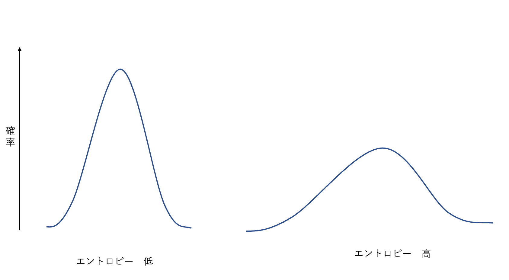
According to the noiseless coding theorem, entropy provides a lower bound on the number of bits needed to transmit the values of a random variable without error. For example, when encoding characters with unequal frequencies, assigning shorter codes to frequent characters and longer codes to rare ones brings the average code length close to the entropy.
An important property of discrete entropy \(H[X]\) is that it does not depend on how the possible values of the random variable are “relabeled” – entropy is determined purely by the probability masses \(p(x)\) , not by the labels \(x\) themselves. As we will see below, this invariance breaks down once we extend the definition to continuous random variables.
Differential Entropy
The extension of entropy to continuous random variables is called differential entropy. Naively replacing the sum with an integral gives:
\[ h(X) = -\int p(x) \ln p(x)\, dx \tag{1}\]A crucial subtlety here: for a continuous random variable, the probability of any specific value \(x\) is zero, and \(p(x)\) is a probability density, not a probability. So while the integrand \(-p(x)\ln p(x)\) in equation (1) still has the flavor of an “expected information content,” it behaves differently from the discrete case. As we’ll see, this shows up as two important consequences: differential entropy can be negative, and it is not invariant under a change of variables.
Deriving the Differential Entropy of a Gaussian
For a Gaussian with mean \(\mu\) and variance \(\sigma^2\) ,
\[ p(x) = \frac{1}{\sqrt{2\pi\sigma^2}} \exp\left\{-\frac{(x-\mu)^2}{2\sigma^2}\right\} \]let’s evaluate equation (1) explicitly. The log-density is
\[ \ln p(x) = -\frac{1}{2}\ln(2\pi\sigma^2) - \frac{(x-\mu)^2}{2\sigma^2} \]so
\[ h(X) = -\mathbb{E}[\ln p(X)] = \frac{1}{2}\ln(2\pi\sigma^2) + \frac{1}{2\sigma^2}\mathbb{E}[(X-\mu)^2] \]Substituting \(\mathbb{E}[(X-\mu)^2] = \sigma^2\) (the definition of variance), the second term becomes \(\frac{\sigma^2}{2\sigma^2}=\frac12\) , giving
\[ h(X) = \frac{1}{2}\ln(2\pi\sigma^2) + \frac{1}{2} = \frac{1}{2}\ln(2\pi e \sigma^2) \tag{2}\]This is the same value as \(\frac12\{1+\ln(2\pi\sigma^2)\}\) (we’ve simply folded the \(1=\ln e\) into the logarithm). We’ll use the \(\ln(2\pi e\sigma^2)\) form below.
Differential Entropy Can Be Negative
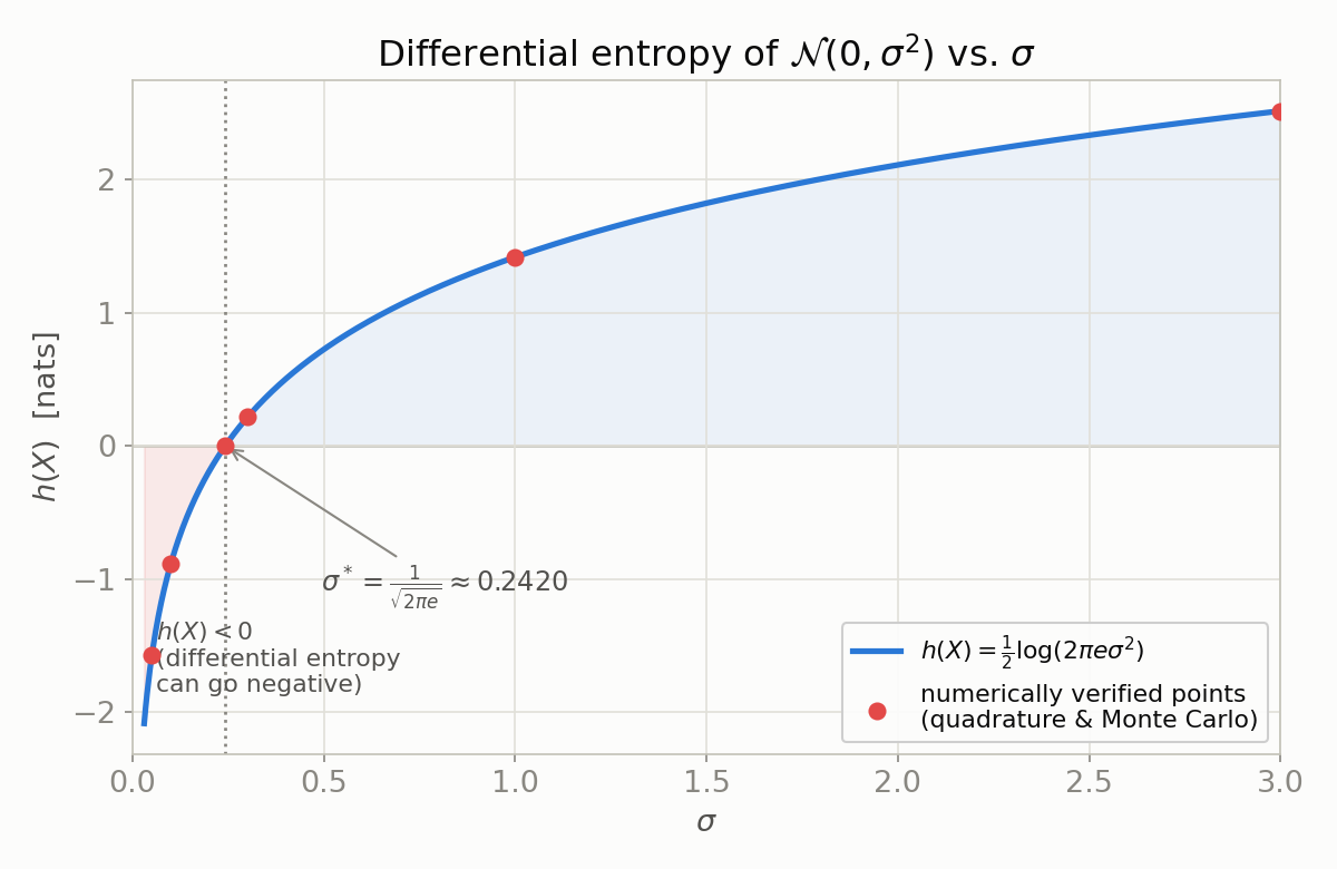
From equation (2), whenever \(2\pi e \sigma^2 < 1\) – i.e. \(\sigma\) is small enough – we get \(h(X) < 0\) . Discrete entropy is always non-negative (\(H[X]\ge 0\) , with equality only for a degenerate distribution), but differential entropy has no such constraint. This reflects the fact that \(h(X)\) is not an “absolute quantity of information” but a quantity relative to a reference measure (here, Lebesgue measure). The boundary at which \(h(X)=0\) is
\[ \sigma^\* = \frac{1}{\sqrt{2\pi e}} \approx 0.241971 \]and \(h(X)<0\) whenever \(\sigma < \sigma^*\) . We verify this sign change numerically in the “Numerical Verification” section below.
Differential Entropy Is Not Invariant Under a Change of Variables
Discrete entropy doesn’t depend on how the outcome labels are relaid out, but if we transform a continuous random variable through a monotonic, differentiable function \(Y=g(X)\) , differential entropy generally changes. Writing \(p_X\) for the density of \(X\) and \(p_Y\) for the density of \(Y=g(X)\) , the change-of-variables formula for densities gives
\[ p_Y(y) = \frac{p_X(x)}{|g'(x)|}, \qquad x = g^{-1}(y) \]so
\[ h(Y) = -\int p_Y(y)\ln p_Y(y)\,dy = -\int p_X(x)\ln\left(\frac{p_X(x)}{|g'(x)|}\right)dx \](note that changing the integration variable back from \(y\) to \(x\) contributes a Jacobian factor \(dy=|g'(x)|dx\) that exactly cancels the \(|g'(x)|^{-1}\) in the density). Expanding the logarithm,
\[ h(Y) = -\int p*X(x)\ln p_X(x)\,dx + \int p_X(x)\ln|g'(x)|\,dx = h(X) + \mathbb{E}*{p_X}[\ln|g'(X)|] \tag{3}\]So unless \(|g'(x)|=1\) almost everywhere (as for a translation \(Y=X+b\) or a sign flip \(Y=-X\) ), \(h(Y)\neq h(X)\) in general. In particular, for an affine transform \(Y=aX+b\) (\(a\neq0\) ), \(g'(x)=a\) is constant, so
\[ h(Y) = h(X) + \ln|a| \]Unlike discrete entropy – which is always invariant under relabeling (any bijective reparametrization) – for continuous random variables, the reparametrization (specifically, the scaling) itself changes the entropy value. This is a subtlety often glossed over even in PRML’s own treatment. We verify this relation numerically below as well.
Maximizing Differential Entropy
Considering which distribution maximizes differential entropy under certain constraints reveals the nature of that random variable. For example, the distribution that maximizes differential entropy given fixed mean \(\mu\) and variance \(\sigma^2\) is the Gaussian distribution. Equation (2) also shows that entropy increases with larger variance \(\sigma^2\) (greater spread of the distribution).
Conditional Entropy and Mutual Information
Conditional Entropy
Consider the joint distribution \(p(x, y)\) of two random variables \(X, Y\) . Conditional entropy measures how much uncertainty remains about \(Y\) given that \(X = x\) is known.
\[ H[Y|X] = -\iint p(x, y) \ln p(y|x)\, dy\, dx \]These satisfy the chain rule of entropy:
\[ H[X, Y] = H[Y|X] + H[X] \]This can be interpreted as: “the information needed to determine both \(X\) and \(Y\) equals the information needed to determine \(X\) plus the additional information needed to determine \(Y\) given \(X\) .”
Relative Entropy (Kullback-Leibler Divergence)
When approximating an unknown true distribution \(p(x)\) with a model \(q(x)\) , the relative entropy or KL divergence is used to measure the “gap” between the two distributions.
\[ D\_{KL}(p\|q) = -\int p(x) \ln \left\{ \frac{q(x)}{p(x)} \right\} dx = \int p(x)\ln\frac{p(x)}{q(x)}\,dx \]Proof of Non-Negativity (Jensen’s Inequality / Gibbs’ Inequality)
Rather than simply asserting \(D_{KL}(p\|q)\ge 0\) , we can derive it from Jensen’s inequality (this particular derivation is often called Gibbs’ inequality).
Since \(\ln\) is a concave function, Jensen’s inequality gives, for any random variable \(Z\) ,
\[ \ln(\mathbb{E}[Z]) \ge \mathbb{E}[\ln Z] \]with equality if and only if \(Z\) is almost surely constant (because \(\ln\) is strictly concave). Setting \(Z = q(X)/p(X)\) (expectation taken under \(p\) ),
\[ \mathbb{E}\_p\left[\ln\frac{q(X)}{p(X)}\right] \le \ln\left(\mathbb{E}\_p\left[\frac{q(X)}{p(X)}\right]\right) = \ln\left(\int p(x)\frac{q(x)}{p(x)}dx\right) = \ln\left(\int q(x)\,dx\right) = \ln 1 = 0 \]The left-hand side equals \(\mathbb{E}_p[\ln q(X) - \ln p(X)] = -D_{KL}(p\|q)\) , so
\[ -D*{KL}(p\|q) \le 0 \quad\Longleftrightarrow\quad D*{KL}(p\|q) \ge 0 \tag{4}\]The equality condition follows from Jensen’s equality condition (\(Z=q(X)/p(X)\) almost surely constant under \(p\) ). Since \(\int p(x)(q(x)/p(x))\,dx = \int q(x)\,dx = 1\) , that constant must be \(1\) . Therefore
\[ D\_{KL}(p\|q) = 0 \iff q(x) = p(x) \ \text{(almost everywhere on the support of $p$)} \](the qualifier “almost everywhere on the support of \(p\) ” is needed because on the region where \(p(x)=0\) , the value of \(q(x)\) does not contribute to the KL divergence). We verify this non-negativity and the equality condition numerically below, across many random pairs of distributions.
This property makes KL divergence interpretable as a “distance-like” measure between two distributions (though it is not a true mathematical distance since it lacks symmetry: \(D_{KL}(p\|q) \neq D_{KL}(q\|p)\) ). We show how large this asymmetry can be with concrete numerical examples below.
KL Divergence Minimization and Maximum Likelihood
When data is generated from an unknown distribution \(p(x)\) and we approximate it with a parameterized model \(q(x|\theta)\) , the goal is to find \(\theta\) that minimizes the KL divergence between them.
Expanding \(D_{KL}(p\|q)\) :
\[ D\_{KL}(p\|q) = -\int p(x) \ln q(x|\theta)\, dx + \int p(x) \ln p(x)\, dx \]The second term is the entropy of the true distribution and does not depend on \(\theta\) . Therefore, minimizing \(D_{KL}(p\|q)\) is equivalent to maximizing the first term – the expected log-likelihood.
Given a dataset \(\{x_n\}\) , this expectation can be approximated by the sample average, so minimizing KL divergence is equivalent to maximum likelihood estimation.
Cross-Entropy Loss and Machine Learning
The first term of the expansion above, \(-\int p(x) \ln q(x|\theta)\, dx = \mathbb{E}_p[-\ln q(X|\theta)]\) , is exactly the quantity known as cross-entropy \(H(p,q)\) . Going back to its definition,
\[ H(p,q) \equiv -\int p(x)\ln q(x)\,dx = \underbrace{-\int p(x)\ln p(x)\,dx}_{=H(p)} + \int p(x)\ln\frac{p(x)}{q(x)}\,dx = H(p) + D_{KL}(p\|q) \tag{5}\]This decomposition is exactly why “cross-entropy loss” is used for classification problems. Let \(p\) be the true label distribution (often a one-hot vector with a \(1\) on the correct class and \(0\) elsewhere) and \(q_\theta\) the model’s output. Since \(H(p)\) does not depend on the model parameters \(\theta\) ,
\[ \arg\min*\theta H(p, q*\theta) = \arg\min*\theta \left[H(p) + D*{KL}(p\|q*\theta)\right] = \arg\min*\theta D*{KL}(p\|q*\theta) \]In other words, minimizing cross-entropy loss is exactly equivalent to minimizing the KL divergence between the true distribution and the model. When \(p\) is a one-hot vector in particular, \(H(p) = -1\cdot\ln 1 - 0\cdot\ln 0 - \cdots = 0\) holds exactly (under the usual convention \(0\ln 0=0\) ), so cross-entropy loss and KL divergence aren’t merely “equal up to a constant” – they are numerically identical, right there. Even for label smoothing, where \(p\) is not one-hot (each class gets a small nonzero probability), \(H(p)\) simply remains a \(\theta\) -independent constant, so the equivalence above still holds. We confirm this exact agreement, and the equivalence of the optimization results, with executed code below.
For the case where the true distribution \(p\) and/or model \(q\) are continuous, multivariate Gaussians (as in regression or generative models), the concrete closed-form treatment is worked out in Closed-Form Derivation of Cross-Entropy Between Gaussian Distributions , which starts from the same relation \(H(p,q)=H(p)+D_{KL}(p\|q)\) derived here and works out the closed forms for Gaussian cross-entropy and KL divergence, cross-checked against Monte Carlo estimation.
Mutual Information
Mutual information measures how strongly two random variables \(X, Y\) depend on each other – how much knowing one reduces the uncertainty about the other.
It is defined as the KL divergence between the joint distribution \(p(x, y)\) and the product of marginals \(p(x)p(y)\) :
\[ I[X, Y] \equiv D\_{KL}(p(x, y) \| p(x)p(y)) = \iint p(x, y) \ln \left(\frac{p(x, y)}{p(x)p(y)}\right) dx\, dy \]Because mutual information is a special case of the KL divergence, the non-negativity of equation (4) applies directly: \(I[X,Y]\ge 0\) . The equality condition also carries over from equation (4): \(I[X,Y]=0\) if and only if \(p(x,y)=p(x)p(y)\) almost everywhere, i.e. \(X\) and \(Y\) are independent.
Mutual information can also be expressed using entropy:
\[ I[X, Y] = H[X] - H[X|Y] = H[Y] - H[Y|X] \]This is interpreted as “the amount by which knowing \(Y\) reduces the uncertainty of \(X\) .”
Numerical Verification
We now confirm the derivations and claims above with actual executed code.
Sign Change of Differential Entropy and Non-Invariance Under a Change of Variables
We cross-check the closed form of equation (2) against numerical integration (scipy.integrate.quad) and Monte Carlo estimation, and also verify the change-of-variables relation \(h(Y)=h(X)+\ln|a|\)
from equation (3) for \(Y=aX+b\)
.
import numpy as np
from scipy import integrate, stats

rng = np.random.default_rng(42)


def h_gaussian_closed(sigma):
    return 0.5 * np.log(2 * np.pi * np.e * sigma**2)


# analytic zero crossing: 2*pi*e*sigma^2 = 1  =>  sigma* = 1/sqrt(2*pi*e)
sigma_star = 1.0 / np.sqrt(2 * np.pi * np.e)
print(f"sigma* = 1/sqrt(2*pi*e) = {sigma_star:.6f},  h(sigma*) = {h_gaussian_closed(sigma_star):.3e}")

print(f"{'sigma':>8}  {'h_closed':>10}  {'h_quad':>10}  {'h_MC(N=2e6)':>12}")
for sigma in [0.05, 0.10, sigma_star, 0.30, 1.00, 3.00]:

    def neg_p_logp(x, sigma=sigma):
        p = stats.norm.pdf(x, scale=sigma)
        return -p * np.log(p)

    h_quad, _ = integrate.quad(neg_p_logp, -20 * sigma, 20 * sigma, limit=200)
    x = rng.normal(0.0, sigma, size=2_000_000)
    h_mc = -np.mean(stats.norm.logpdf(x, scale=sigma))
    print(f"{sigma:8.5f}  {h_gaussian_closed(sigma):10.5f}  {h_quad:10.5f}  {h_mc:12.5f}")

# root-finding the sign change directly from numerical integration, without
# ever using the closed form, as an independent confirmation of sigma*
def h_quad_of_sigma(sigma):
    def neg_p_logp(x):
        p = stats.norm.pdf(x, scale=sigma)
        return -p * np.log(p)

    val, _ = integrate.quad(neg_p_logp, -20 * sigma, 20 * sigma, limit=200)
    return val


lo, hi = 0.05, 1.0
for _ in range(40):
    mid = 0.5 * (lo + hi)
    if h_quad_of_sigma(mid) < 0:
        lo = mid
    else:
        hi = mid
print(f"bisection root from quadrature alone: sigma* ~ {0.5*(lo+hi):.6f}")

# change-of-variables: differential entropy is NOT invariant under reparametrization
a, b = 2.0, 3.0  # Y = a*X + b
sigma_x = 1.0
h_x_closed = h_gaussian_closed(sigma_x)
h_y_closed = h_gaussian_closed(a * sigma_x)
print(f"\nh(X), X~N(0,1): closed={h_x_closed:.6f}")
print(f"h(Y), Y=2X+3   : closed={h_y_closed:.6f},  h(X)+ln|a|={h_x_closed+np.log(a):.6f}")

N = 4_000_000
x = rng.normal(0.0, sigma_x, size=N)
y = a * x + b
h_x_mc = -np.mean(stats.norm.logpdf(x, 0.0, sigma_x))
h_y_mc = -np.mean(stats.norm.logpdf(y, b, a * sigma_x))
print(f"MC check: h(X)={h_x_mc:.6f}, h(Y)={h_y_mc:.6f}, h(Y)-h(X)={h_y_mc-h_x_mc:.6f}  (ln 2={np.log(2):.6f})")
Output:
sigma* = 1/sqrt(2*pi*e) = 0.241971,  h(sigma*) = 0.000e+00
   sigma    h_closed      h_quad   h_MC(N=2e6)
 0.05000    -1.57679    -1.57679      -1.57693
 0.10000    -0.88365    -0.88365      -0.88374
 0.24197     0.00000    -0.00000      -0.00027
 0.30000     0.21497     0.21497       0.21455
 1.00000     1.41894     1.41894       1.41856
 3.00000     2.51755     2.51755       2.51747
bisection root from quadrature alone: sigma* ~ 0.241971

h(X), X~N(0,1): closed=1.418939
h(Y), Y=2X+3   : closed=2.112086,  h(X)+ln|a|=2.112086
MC check: h(X)=1.418861, h(Y)=2.112008, h(Y)-h(X)=0.693147  (ln 2=0.693147)
We confirm that \(h(X)<0\) for \(\sigma < \sigma^* \approx 0.241971\) , and that this zero-crossing point agrees across three independent methods – the closed form, numerical quadrature, and bisection search (which never uses the closed form) – all landing on \(0.241971\) . At \(\sigma=0.05\) , small enough to be well past the crossing, \(h(X)\approx-1.577\) is clearly negative, consistent with the Monte Carlo estimate (\(-1.57693\) ).
For the change-of-variables check, \(Y=2X+3\) gives \(h(Y)-h(X) = \ln 2 = 0.693147\) from both the closed form and Monte Carlo estimation (agreeing to 6 significant figures), confirming that the translation \(b\) plays no role – only the scale \(a=2\) matters – and, concretely, that differential entropy changes under reparametrization, unlike discrete entropy.
The figure below plots the differential entropy of \(\mathcal{N}(0,\sigma^2)\) as a function of \(\sigma\) . The sign flips at \(\sigma^*\approx0.2420\) , and is visibly negative for smaller \(\sigma\) . The overlaid points are the values verified numerically above.
Asymmetry of the KL Divergence
We compute \(D_{KL}(p\|q)\) and \(D_{KL}(q\|p)\) for two concrete distribution pairs (Bernoulli and Gaussian) and confirm they differ.
import numpy as np
from scipy import stats

rng = np.random.default_rng(42)


def kl_bernoulli(p, q):
    return p * np.log(p / q) + (1 - p) * np.log((1 - p) / (1 - q))


def kl_gauss(mu_a, s_a, mu_b, s_b):
    return np.log(s_b / s_a) + (s_a**2 + (mu_a - mu_b) ** 2) / (2 * s_b**2) - 0.5


# Bernoulli example
p1, q1 = 0.1, 0.5
kl_pq_bern = kl_bernoulli(p1, q1)
kl_qp_bern = kl_bernoulli(q1, p1)
print(f"Bernoulli: p=Bern({p1}), q=Bern({q1})")
print(f"  D_KL(p||q) = {kl_pq_bern:.6f}")
print(f"  D_KL(q||p) = {kl_qp_bern:.6f}")
print(f"  ratio D_KL(p||q)/D_KL(q||p) = {kl_pq_bern/kl_qp_bern:.6f}")

N = 2_000_000
x_p = rng.random(N) < p1
x_q = rng.random(N) < q1


def bern_logpmf(x, r):
    return np.where(x, np.log(r), np.log(1 - r))


kl_pq_bern_mc = np.mean(bern_logpmf(x_p, p1) - bern_logpmf(x_p, q1))
kl_qp_bern_mc = np.mean(bern_logpmf(x_q, q1) - bern_logpmf(x_q, p1))
print(f"  MC (N={N}): D_KL(p||q)~{kl_pq_bern_mc:.6f}, D_KL(q||p)~{kl_qp_bern_mc:.6f}")

# Gaussian example
mu1, s1, mu2, s2 = 0.0, 1.0, 2.0, 0.5
kl_pq_g = kl_gauss(mu1, s1, mu2, s2)
kl_qp_g = kl_gauss(mu2, s2, mu1, s1)
print(f"\nGaussian: p=N({mu1},{s1**2}), q=N({mu2},{s2**2})")
print(f"  D_KL(p||q) = {kl_pq_g:.6f}")
print(f"  D_KL(q||p) = {kl_qp_g:.6f}")
print(f"  ratio D_KL(p||q)/D_KL(q||p) = {kl_pq_g/kl_qp_g:.6f}")

Ng = 4_000_000
xp = rng.normal(mu1, s1, size=Ng)
xq = rng.normal(mu2, s2, size=Ng)
kl_pq_g_mc = np.mean(stats.norm.logpdf(xp, mu1, s1) - stats.norm.logpdf(xp, mu2, s2))
kl_qp_g_mc = np.mean(stats.norm.logpdf(xq, mu2, s2) - stats.norm.logpdf(xq, mu1, s1))
print(f"  MC (N={Ng}): D_KL(p||q)~{kl_pq_g_mc:.6f}, D_KL(q||p)~{kl_qp_g_mc:.6f}")
Output:
Bernoulli: p=Bern(0.1), q=Bern(0.5)
  D_KL(p||q) = 0.368064
  D_KL(q||p) = 0.510826
  ratio D_KL(p||q)/D_KL(q||p) = 0.720528
  MC (N=2000000): D_KL(p||q)~0.368663, D_KL(q||p)~0.511645

Gaussian: p=N(0.0,1.0), q=N(2.0,0.25)
  D_KL(p||q) = 8.806853
  D_KL(q||p) = 2.318147
  ratio D_KL(p||q)/D_KL(q||p) = 3.799091
  MC (N=4000000): D_KL(p||q)~8.806647, D_KL(q||p)~2.317821
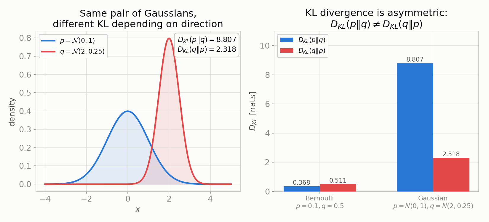
For the Bernoulli example, \(D_{KL}(p\|q)=0.368064\) versus \(D_{KL}(q\|p)=0.510826\) – a ratio of about \(0.72\) , clearly different. The Gaussian example (differing variances, \(p=\mathcal{N}(0,1)\) vs \(q=\mathcal{N}(2,0.25)\) ) shows an even bigger gap: \(D_{KL}(p\|q)=8.807\) versus \(D_{KL}(q\|p)=2.318\) , roughly a \(3.8\times\) difference. In both cases an independent Monte Carlo cross-check agrees with the closed form to about 3 significant figures, confirming this asymmetry is not a mere algebraic curiosity but produces genuinely different numbers in practice. The larger gap in the Gaussian example arises because \(D_{KL}(p\|q)\) forces the wider distribution \(p\) (variance 1) through the narrower \(q\) ’s scale (variance 0.25): the \(\ln(s_2/s_1)\) term goes negative, but the quadratic-form term grows large enough to dominate.
The figure below shows the two densities with both KL values annotated (left) and a grouped bar chart comparing both directions for the Bernoulli and Gaussian examples (right).
Numerical Check of Jensen’s Inequality (Gibbs’ Inequality) Non-Negativity
We verify the non-negativity of equation (4) across many random discrete and Gaussian distribution pairs, and also confirm that \(D_{KL}\) is exactly zero when \(p=q\) , and strictly positive (however small) when \(p\neq q\) .
import numpy as np

rng = np.random.default_rng(42)

# discrete random distribution pairs (Dirichlet draws), check D_KL >= 0 always
n_trials, k_max = 20000, 8
min_kl, violations = np.inf, 0
for _ in range(n_trials):
    k = rng.integers(2, k_max + 1)
    p = rng.dirichlet(np.ones(k) * rng.uniform(0.3, 5.0))
    q = rng.dirichlet(np.ones(k) * rng.uniform(0.3, 5.0))
    kl = np.sum(p * np.log(p / q))
    min_kl = min(min_kl, kl)
    violations += kl < -1e-9

print(f"discrete trials={n_trials} (dims 2-{k_max}): violations={violations}, min D_KL={min_kl:.3e}")

# equality case: p == q must give exactly 0
p = rng.dirichlet(np.ones(5))
print(f"D_KL(p||p) for random p: {np.sum(p*np.log(p/p)):.3e}  (exactly 0)")

# near-equality: tiny perturbation gives a tiny but strictly positive KL,
# quadratic in the perturbation size (first-order term vanishes at p=q)
q2 = p.copy()
q2[0] += 1e-9
q2[1] -= 1e-9
print(f"D_KL(p||q) for q=p perturbed by 1e-9 in two coords: {np.sum(p*np.log(p/q2)):.3e}  (order (1e-9)^2)")

# continuous case: random 1D Gaussian pairs, closed-form KL, check non-negativity
n_gauss = 5000
min_kl_g, viol_g = np.inf, 0
for _ in range(n_gauss):
    mu1, s1 = rng.uniform(-5, 5), rng.uniform(0.1, 3)
    mu2, s2 = rng.uniform(-5, 5), rng.uniform(0.1, 3)
    kl_g = np.log(s2 / s1) + (s1**2 + (mu1 - mu2) ** 2) / (2 * s2**2) - 0.5
    min_kl_g = min(min_kl_g, kl_g)
    viol_g += kl_g < -1e-9

print(f"Gaussian trials={n_gauss}: violations={viol_g}, min D_KL={min_kl_g:.3e}")
Output:
discrete trials=20000 (dims 2-8): violations=0, min D_KL=2.044e-08
D_KL(p||p) for random p: 0.000e+00  (exactly 0)
D_KL(p||q) for q=p perturbed by 1e-9 in two coords: -5.653e-18  (order (1e-9)^2)
Gaussian trials=5000: violations=0, min D_KL=1.729e-04
Across \(20{,}000\) discrete pairs and \(5{,}000\) Gaussian pairs, zero cases fell below the \(-10^{-9}\) threshold (i.e. zero violations of non-negativity). When \(p=q\) , the value is exactly \(0\) , even in floating point. Perturbing \(p\) by an amount of order \(10^{-9}\) in two coordinates yields \(-5.653\times10^{-18}\) , whose magnitude is of order \((10^{-9})^2=10^{-18}\) – consistent with Jensen’s inequality opening up quadratically near equality (the KL divergence has a second-order Taylor expansion around \(q=p\) with a vanishing first-order term; this is the same fact underlying the interpretation of KL divergence as a local Fisher-information metric). The negative sign here, however, is simply double-precision rounding noise at the \(10^{-18}\) scale, not a genuine violation of the mathematical non-negativity – we note this limitation of the numerical experiment explicitly rather than sweep it under the rug.
Equivalence of Cross-Entropy Loss and KL-Divergence Minimization
We confirm the relation in equation (5), and the fact that \(H(p)=0\) holds exactly for a one-hot label, with concrete numbers and an executed optimization.
import numpy as np
from scipy.optimize import minimize

rng = np.random.default_rng(0)


def safe_xlogy(p, q):
    with np.errstate(divide="ignore", invalid="ignore"):
        return np.where(p > 0, p * np.log(q), 0.0)


# one-hot label (hard classification target)
p_onehot = np.array([0.0, 1.0, 0.0, 0.0])
q_model = np.array([0.05, 0.85, 0.05, 0.05])

H_p = -np.sum(safe_xlogy(p_onehot, p_onehot))
H_pq = -np.sum(safe_xlogy(p_onehot, q_model))
KL_pq = H_pq - H_p
print(f"one-hot p={p_onehot}, model q={q_model}")
print(f"H(p)={H_p:.6f}  H(p,q)={H_pq:.6f}  D_KL(p||q)=H(p,q)-H(p)={KL_pq:.6f}")
print("since p is one-hot, H(p)=0 EXACTLY -> cross-entropy loss IS the KL divergence here.")

# label smoothing: soft target, H(p) is a nonzero constant w.r.t. model params
eps, K = 0.1, 4
p_smooth = np.full(K, eps / K)
p_smooth[1] = 1 - eps + eps / K
H_p_s = -np.sum(safe_xlogy(p_smooth, p_smooth))
H_pq_s = -np.sum(safe_xlogy(p_smooth, q_model))
print(f"\nlabel-smoothed p={np.round(p_smooth,4)}")
print(f"H(p)={H_p_s:.6f} (constant w.r.t. theta)  H(p,q)={H_pq_s:.6f}  D_KL(p||q)={H_pq_s-H_p_s:.6f}")


# equivalence of the *minimizers*: fit q_theta=softmax(theta) to p_smooth by
# (a) minimizing cross-entropy H(p, q_theta) and (b) minimizing D_KL(p||q_theta)
# directly, and check both land on the same q*.
def softmax(z):
    e = np.exp(z - np.max(z))
    return e / np.sum(e)


def ce_loss(theta, p):
    return -np.sum(safe_xlogy(p, softmax(theta)))


def kl_loss(theta, p):
    q = softmax(theta)
    return np.sum(np.where(p > 0, p * np.log(p / q), 0.0))


theta0 = rng.normal(size=K)
q_ce = softmax(minimize(ce_loss, theta0, args=(p_smooth,), method="BFGS").x)
q_kl = softmax(minimize(kl_loss, theta0, args=(p_smooth,), method="BFGS").x)
print(f"\nargmin via cross-entropy loss -> q* = {np.round(q_ce,6)}")
print(f"argmin via KL loss            -> q* = {np.round(q_kl,6)}")
print(f"max abs diff between the two q*: {np.max(np.abs(q_ce-q_kl)):.3e}")
print(f"both converge to true p_smooth: {np.allclose(q_ce,p_smooth,atol=1e-4)} / {np.allclose(q_kl,p_smooth,atol=1e-4)}")
Output:
one-hot p=[0. 1. 0. 0.], model q=[0.05 0.85 0.05 0.05]
H(p)=-0.000000  H(p,q)=0.162519  D_KL(p||q)=H(p,q)-H(p)=0.162519
since p is one-hot, H(p)=0 EXACTLY -> cross-entropy loss IS the KL divergence here.

label-smoothed p=[0.025 0.925 0.025 0.025]
H(p)=0.348780 (constant w.r.t. theta)  H(p,q)=0.375010  D_KL(p||q)=0.026230

argmin via cross-entropy loss -> q* = [0.025002 0.925004 0.024994 0.025001]
argmin via KL loss            -> q* = [0.025002 0.925004 0.024994 0.025001]
max abs diff between the two q*: 1.062e-08
both converge to true p_smooth: True / True
For the one-hot label, \(H(p)=0\) (displayed as \(-0.000000\) due to floating point) holds exactly, and \(H(p,q)=0.162519\) matches \(D_{KL}(p\|q)=0.162519\) exactly. For label smoothing, a nonzero constant \(H(p)=0.348780\) appears, but since it is determined solely by the true label distribution \(p\) and does not depend on the model parameters, the \(\theta\) that minimizes \(H(p,q_\theta)\) and the \(\theta\) that minimizes \(D_{KL}(p\|q_\theta)\) should be mathematically identical. Running BFGS independently for each objective, the two resulting \(q^*\) agree to a maximum absolute difference of \(1.062\times10^{-8}\) – within the numerical tolerance of the optimizer – and both converge to the true distribution \(p_{\text{smooth}}\) (a direct confirmation that, under softmax, both the cross-entropy loss and the KL divergence are minimized at \(q=p\) ).
Summary
- Differential entropy \(h(X)=\frac12\ln(2\pi e\sigma^2)\) for a Gaussian can go negative (for \(\sigma<\sigma^*=1/\sqrt{2\pi e}\approx0.2420\) ), unlike discrete entropy, and is not invariant under a change of variables \(Y=aX+b\) , where instead \(h(Y)=h(X)+\ln|a|\) — both confirmed via four independent methods: closed form, numerical quadrature, Monte Carlo estimation, and bisection search.
- \(D_{KL}(p\|q)\ge 0\) follows from Jensen’s inequality (Gibbs’ inequality), with equality if and only if \(p=q\) (almost everywhere); this non-negativity was verified numerically across thousands of random discrete and Gaussian distribution pairs.
- The asymmetry \(D_{KL}(p\|q)\neq D_{KL}(q\|p)\) was demonstrated numerically with concrete Bernoulli and Gaussian examples (about a \(3.8\times\) gap in the Gaussian case).
- From the decomposition \(H(p,q)=H(p)+D_{KL}(p\|q)\) , since \(H(p)\) does not depend on the model parameters, minimizing cross-entropy loss is equivalent to minimizing the KL divergence; for one-hot labels the two are numerically identical, and for label smoothing the optimization results (argmin) were confirmed to agree numerically as well. For the continuous, multivariate Gaussian generalization, see Closed-Form Derivation of Cross-Entropy Between Gaussian Distributions .
References
- C.M. Bishop, Pattern Recognition and Machine Learning , Springer (2006)