Introduction
The basics of Particle Swarm Optimization (PSO), along with the stability analysis around inertia weight and the constriction coefficient, were covered in detail in The Mathematics of PSO and its Python Implementation . The key conclusion there was that PSO is prone to premature convergence: since every particle is pulled toward the single global best \(\mathbf{g}\) , the swarm loses diversity early and stagnates near local optima.
This article covers Two-swarm Cooperative PSO (TCPSO), proposed by Sun & Li (2013) to address exactly this diversity-loss problem. TCPSO coordinates two particle swarms with distinct roles — a slave swarm responsible for fast convergence and a master swarm responsible for maintaining diversity — and is reported to find the global optimum even in extremely wide search spaces (the original paper demonstrates a search interval on the order of \(2 \times 10^{10}\) ).
Rather than simply restating the update rules as given (as the previous version of this article did), we focus on three things:
- Deriving, from linear stability analysis, exactly why and under what conditions the slave and master swarm velocity update rules converge
- Re-implementing everything in Python and running it with fixed seeds to check, with concrete numbers, under which conditions the textbook story (“slave converges fast, master preserves diversity”) actually holds — and under which conditions it breaks down
- Situating TCPSO within research published since 2023
A Brief Recap of Standard PSO
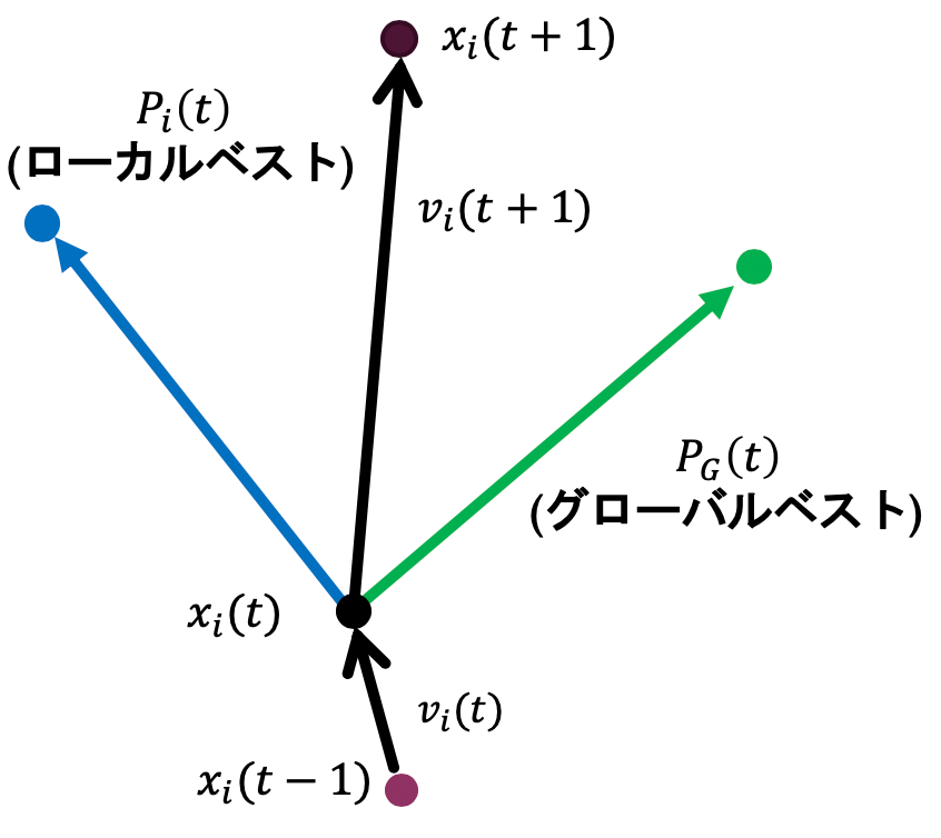
For particle \(i\) with position \(x_i(t)\) , velocity \(v_i(t)\) , personal best \(P_i(t)\) , and global best \(P_G(t)\) , the standard PSO update rules are:
\[ v_i(t+1) = w \cdot v_i(t) + C_1 r_1 (P_i(t) - x_i(t)) + C_2 r_2 (P_G(t) - x_i(t)) \] \[ x_i(t+1) = x_i(t) + v_i(t+1) \]- \(w\) : inertia weight (how much of the current velocity is retained)
- \(C_1, C_2\) : cognitive and social coefficients
- \(r_1, r_2 \sim U[0,1]\) : uniform random numbers
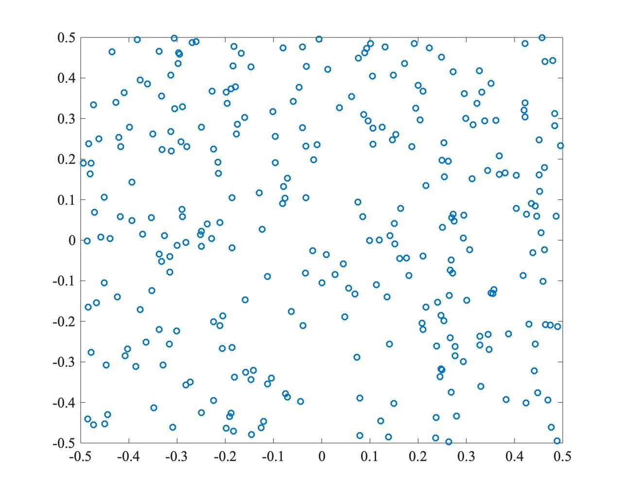
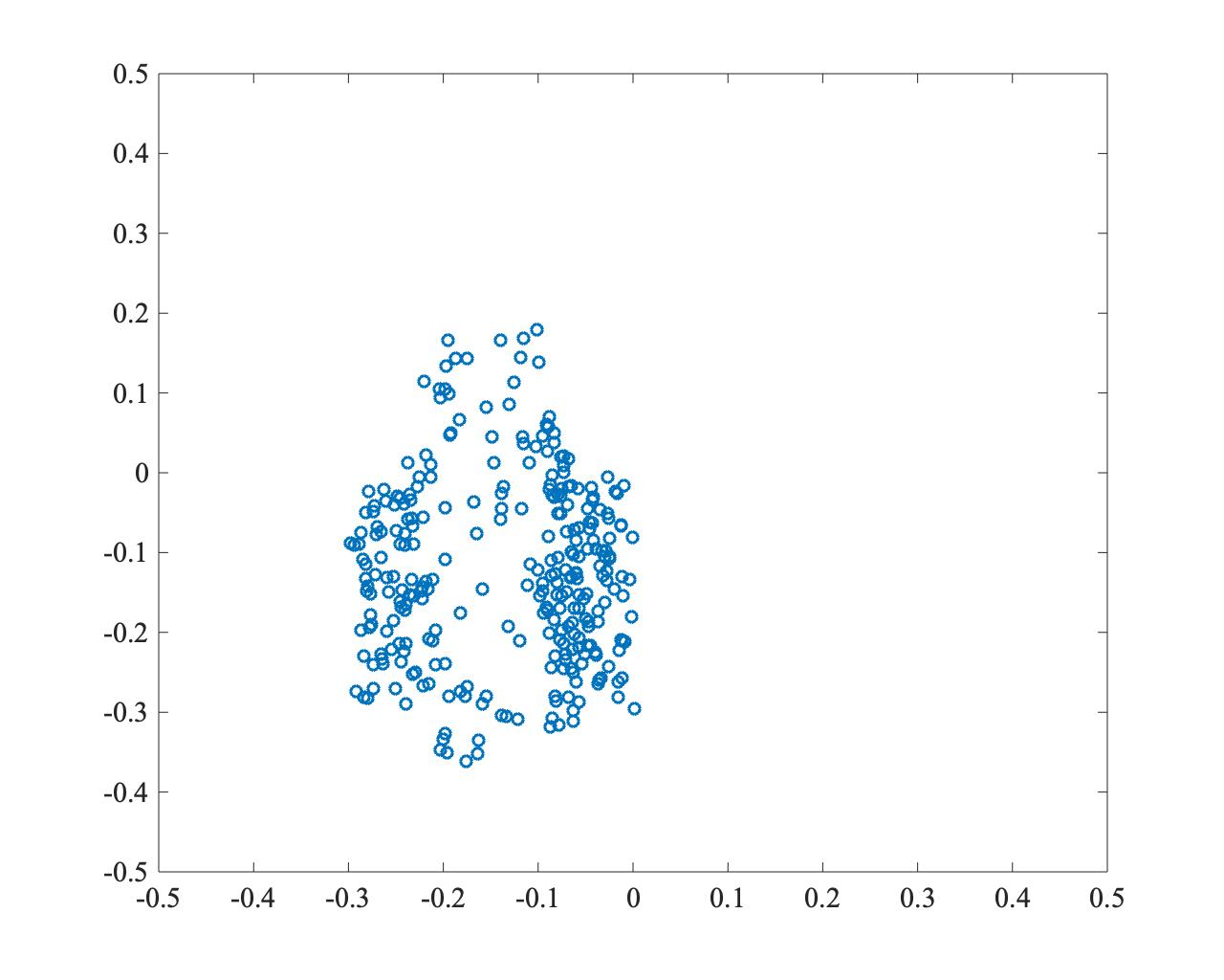
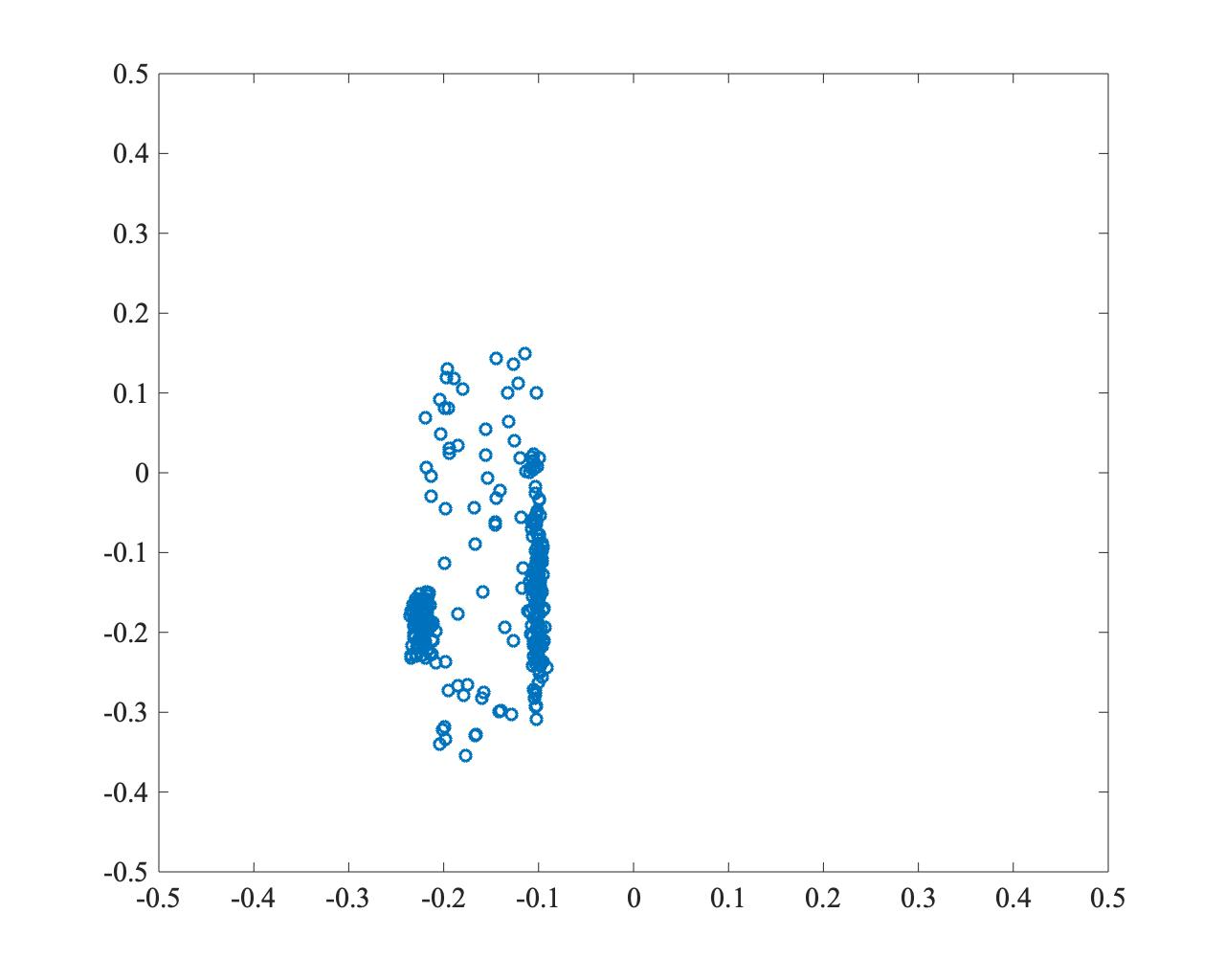
The example below shows PSO searching for the optimal solution at \((0,0)\) . Convergence is fast, but the particles concentrate at a single point, illustrating the local-optima problem (for the full derivation of the relationship between inertia weight/coefficients and convergence/divergence, see The Mathematics of PSO and its Python Implementation ).
- \(t=0\)
- \(t=250\)
- \(t=500\)
Two-Swarm Cooperative PSO (TCPSO)
TCPSO’s key feature is the use of two particle swarms with different roles: a master swarm for global exploration and a slave swarm for intensive local search.
Particle Update Rules
Slave Swarm The slave swarm has no inertia term \(w\) and is strongly attracted to the global best \(P_G(t)\) . This gives it the role of intensively exploring promising regions.
\[ v_i^S(t+1) = C_1^S r_1 (P_i^S(t) - x_i^S(t)) + C_2^S r_2 (P_G(t) - x_i^S(t)) \] \[ x_i^S(t+1) = x_i^S(t) + v_i^S(t+1) \]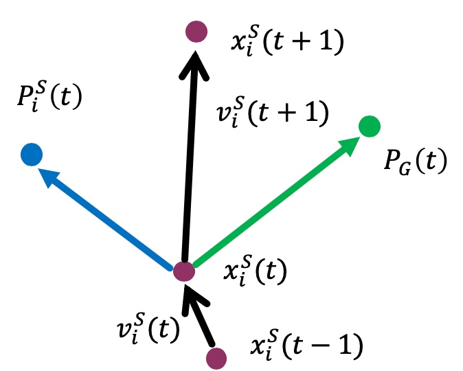
Master Swarm The master swarm also uses the slave swarm’s best position \(P_G^S(t)\) . This allows it to reference promising regions found by the slave swarm while maintaining search diversity through its inertia term.
\[ v_i^M(t+1) = w^M v_i^M(t) + C_1^M r_1 (P_i^M(t) - x_i^M(t)) + C_2^M r_2 (P_G^S(t) - x_i^M(t)) + C_3^M r_3 (P_G(t) - x_i^M(t)) \] \[ x_i^M(t+1) = x_i^M(t) + v_i^M(t+1) \]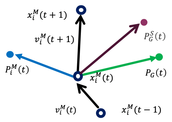
The goal of TCPSO is to combine the slave swarm’s fast convergence with the master swarm’s diversity maintenance. We now derive precisely why this works at the level of the update equations.
Deriving Convergence Conditions
We apply the same technique used for standard PSO’s stability analysis ( The Mathematics of PSO and its Python Implementation, §Stability Analysis ) — reducing to one dimension and one particle, treating pbest/gbest as fixed at a point \(p\) (a local-stagnation regime), and replacing the random numbers with their expectation \(0.5\) — to both the slave and master swarms.
Slave Swarm: A First-Order Recursion and “Deadbeat” Convergence
The slave swarm has no inertia term. Defining the deviation \(e_t = x_t - p\) , and approximating \(P_i^S(t) = P_G(t) = p\) (a locally stagnant regime) with \(r_1, r_2 \to 0.5\) :
\[ v_{t+1} = C_1^S r_1 (p - x_t) + C_2^S r_2 (p - x_t) \to -\phi^S e_t, \qquad \phi^S = \frac{C_1^S + C_2^S}{2} \] \[ e_{t+1} = e_t + v_{t+1} = (1 - \phi^S)\, e_t \tag{S1} \]This is a first-order linear recursion (in contrast to standard PSO and the master swarm, which are second-order systems in velocity and deviation, the inertia-free slave swarm degenerates to a single state \(e_t\) ). The stability condition is simply:
\[ |1 - \phi^S| < 1 \iff 0 < \phi^S < 2 \iff 0 < C_1^S + C_2^S < 4 \tag{S2} \]More interestingly, when \(\phi^S = 1\) (e.g. \(C_1^S = C_2^S = 1.0\) ), the deterministic approximation gives \(e_{t+1} = 0\) — the deviation vanishes in exactly one step (a “deadbeat” response, in control-theory terms). The values \(C_1^S = C_2^S = 1.0\) used in this article’s implementation coincide exactly with this theoretically fastest convergence point.
Master Swarm: A Second-Order Recursion with a Generalized Stability Region
The master swarm has an inertia term and three attraction terms (personal pbest, slave swarm’s gbest, and overall gbest). Approximating \(P_i^M(t) = P_G^S(t) = P_G(t) = p\) and \(r_1, r_2, r_3 \to 0.5\) :
\[ v_{t+1} = w^M v_t - \phi^M e_t, \qquad \phi^M = \frac{C_1^M + C_2^M + C_3^M}{2} \] \[ e_{t+1} = e_t + v_{t+1} = w^M v_t + (1 - \phi^M)\, e_t \]In matrix form, this is structurally identical to the standard PSO second-order system:
$$ \begin{pmatrix} v_{t+1} \ e_{t+1} \end{pmatrix}
\begin{pmatrix} w^M & -\phi^M \ w^M & 1-\phi^M \end{pmatrix} \begin{pmatrix} v_t \ e_t \end{pmatrix} \tag{M1} $$
Applying the Jury stability criterion to the characteristic equation \(\lambda^2 - (1+w^M-\phi^M)\lambda + w^M = 0\) (the derivation is identical to standard PSO, so we omit the details) gives:
\[ w^M < 1, \qquad 0 < C_1^M + C_2^M + C_3^M < 4(1 + w^M) \tag{M2} \]This is a natural generalization of standard PSO’s stability condition \(0 < C_1+C_2 < 4(1+w)\) , where the “sum of coefficients” is simply replaced by the sum of three terms \(C_1^M+C_2^M+C_3^M\) . Comparing (S2) and (M2), the upper bound of the slave swarm’s stability region (\(\phi^S<2\) , i.e. \(C_1^S+C_2^S<4\) ) coincides with the master swarm’s stability bound in the limit \(w^M=0\) (i.e. \(C_1^M+C_2^M+C_3^M<4\) ). In other words, the slave swarm can be understood as a special case of the master swarm with the inertia term fixed to zero.
Numerical Verification
We implement the simplified stagnation models (S1) and (M1) directly and track \(|e_t|\) when random numbers are actually redrawn at every step.
import numpy as np


def simulate_slave_deviation(c1s, c2s, T=60, seed=0, e0=1.0):
    """First-order slave-swarm stagnation model (Eq. S1).
    v_{t+1} = c1s*r1*(p-x_t) + c2s*r2*(p-x_t) = -(c1s r1 + c2s r2) e_t
    e_{t+1} = (1 - c1s r1 - c2s r2) e_t
    """
    rng = np.random.default_rng(seed)
    e = e0
    traj = [abs(e)]
    for _ in range(T):
        r1, r2 = rng.random(), rng.random()
        e = (1 - c1s * r1 - c2s * r2) * e
        traj.append(abs(e) + 1e-300)
    return np.array(traj)


def simulate_master_deviation(w, c1m, c2m, c3m, T=150, seed=0, e0=1.0):
    """Second-order master-swarm stagnation model (Eq. M1); same form as
    standard PSO but phi is the sum of three coefficients."""
    rng = np.random.default_rng(seed)
    v, e = 0.0, e0
    traj = [abs(e)]
    for _ in range(T):
        r1, r2, r3 = rng.random(), rng.random(), rng.random()
        v = w * v - (c1m * r1 + c2m * r2 + c3m * r3) * e
        e = e + v
        traj.append(abs(e) + 1e-300)
    return np.array(traj)


# Slave swarm: convergence speed at the deadbeat point (c1s=c2s=1.0)
n_to_thresh = []
for seed in range(200):
    traj = simulate_slave_deviation(1.0, 1.0, T=60, seed=seed)
    idx = next((i for i, v in enumerate(traj) if v < 1e-6), None)
    if idx is not None:
        n_to_thresh.append(idx)
print(f"iterations to |e_t|<1e-6 (200 seeds): "
      f"mean={np.mean(n_to_thresh):.2f} median={np.median(n_to_thresh):.1f} max={np.max(n_to_thresh)}")

# Master swarm: stochastic divergence can occur even within the nominal bound
configs = [
    ("w=0.9, C1m=C2m=C3m=1.0", 0.9, 1.0, 1.0, 1.0),
    ("w=0.9, C1m=C2m=C3m=1.5 (within bound)", 0.9, 1.5, 1.5, 1.5),
    ("w=0.9, C1m=C2m=C3m=2.0 (beyond bound)", 0.9, 2.0, 2.0, 2.0),
]
for label, w, c1m, c2m, c3m in configs:
    bound = 4 * (1 + w)
    s = c1m + c2m + c3m
    finals = [simulate_master_deviation(w, c1m, c2m, c3m, T=150, seed=s_)[-1] for s_ in range(50)]
    print(f"{label:38} sum={s:.2f} bound={bound:.2f} median|e_150|={np.median(finals):.3e}")
The results are:
iterations to |e_t|<1e-6 (200 seeds): mean=10.06 median=10.0 max=17
w=0.9, C1m=C2m=C3m=1.0                sum=3.00 bound=7.60 median|e_150|=4.238e-02
w=0.9, C1m=C2m=C3m=1.5 (within bound) sum=4.50 bound=7.60 median|e_150|=1.964e+01
w=0.9, C1m=C2m=C3m=2.0 (beyond bound) sum=6.00 bound=7.60 median|e_150|=8.780e+07
At the deadbeat point \(C_1^S=C_2^S=1.0\) , the slave swarm reaches \(|e_t|<10^{-6}\) in a median of just 10 iterations across 200 seeds. The master swarm, meanwhile, diverges to a median of \(19.6\) over 50 seeds even though \(C_1^M+C_2^M+C_3^M=4.5\) lies inside the nominal stability bound \(4(1+w^M)=7.6\) . This is the same phenomenon observed in The Mathematics of PSO and its Python Implementation : the expectation-based bound (M2) is only a rough necessary condition, and it is insufficient to prevent stochastic variance divergence (Jiang, Luo & Yang 2007; Poli 2009; Cleghorn & Engelbrecht 2014). In practice, it is safer to choose coefficient sums well below the nominal bound.
Python Implementation
We re-implement the update rules from the original paper for minimization problems (the original Matlab implementation maximized a fitness value 1/(|x|+|y|); here we rewrite it in a form directly applicable to standard minimization benchmarks).
import numpy as np


def run_tcpso(objective, dim, ns=20, nm=20, max_iter=200, bounds=(-5.12, 5.12),
              w_max=0.9, w_min=0.4, c1s=1.0, c2s=1.0,
              c1m=1.0, c2m=1.0, c3m=1.0, v_max_ratio=0.2, seed=0):
    """TCPSO (Two-swarm Cooperative PSO). The slave swarm has no inertia and
    converges strongly toward gbest; the master swarm uses inertia plus the
    slave's gbest and the overall gbest to keep exploring."""
    rng = np.random.default_rng(seed)
    low, high = bounds
    v_max = v_max_ratio * (high - low)

    # initialize slave swarm
    sp = rng.uniform(low, high, (ns, dim))
    sp_v = np.zeros((ns, dim))
    sp_f = objective(sp)
    sp_best, sp_best_f = sp.copy(), sp_f.copy()
    s_idx = int(np.argmin(sp_best_f))
    s_gbest, s_gbest_f = sp_best[s_idx].copy(), float(sp_best_f[s_idx])

    # initialize master swarm
    mp = rng.uniform(low, high, (nm, dim))
    mp_v = np.zeros((nm, dim))
    mp_f = objective(mp)
    mp_best, mp_best_f = mp.copy(), mp_f.copy()

    m_idx = int(np.argmin(mp_best_f))
    g_best = mp_best[m_idx].copy() if mp_best_f[m_idx] < s_gbest_f else s_gbest.copy()
    g_best_f = min(float(mp_best_f[m_idx]), s_gbest_f)

    history = [g_best_f]
    for t in range(max_iter):
        w = w_max - (w_max - w_min) * (t / max_iter)  # LDIW applied to the master swarm only

        sp_f = objective(sp)
        mp_f = objective(mp)

        # STEP: update pbest
        imp_s = sp_f < sp_best_f
        sp_best[imp_s], sp_best_f[imp_s] = sp[imp_s], sp_f[imp_s]
        imp_m = mp_f < mp_best_f
        mp_best[imp_m], mp_best_f[imp_m] = mp[imp_m], mp_f[imp_m]

        # STEP: update slave gbest / overall gbest
        s_idx = int(np.argmin(sp_best_f))
        if sp_best_f[s_idx] < s_gbest_f:
            s_gbest_f, s_gbest = float(sp_best_f[s_idx]), sp_best[s_idx].copy()
        m_idx = int(np.argmin(mp_best_f))
        if mp_best_f[m_idx] < g_best_f:
            g_best_f, g_best = float(mp_best_f[m_idx]), mp_best[m_idx].copy()
        if s_gbest_f < g_best_f:
            g_best_f, g_best = s_gbest_f, s_gbest.copy()

        # STEP: update slave swarm (no inertia term, Eq. 1)
        r1s, r2s = rng.random((ns, dim)), rng.random((ns, dim))
        sp_v = c1s * r1s * (sp_best - sp) + c2s * r2s * (g_best - sp)
        sp_v = np.clip(sp_v, -v_max, v_max)
        sp = np.clip(sp + sp_v, low, high)

        # STEP: update master swarm (with inertia, Eq. 2)
        r1m, r2m, r3m = rng.random((nm, dim)), rng.random((nm, dim)), rng.random((nm, dim))
        mp_v = (w * mp_v + c1m * r1m * (mp_best - mp)
                + c2m * r2m * (s_gbest - mp) + c3m * r3m * (g_best - mp))
        mp_v = np.clip(mp_v, -v_max, v_max)
        mp = np.clip(mp + mp_v, low, high)

        history.append(g_best_f)

    return g_best, g_best_f, history


def rastrigin(x):
    return 10 * x.shape[-1] + np.sum(x**2 - 10 * np.cos(2 * np.pi * x), axis=-1)


_, best, hist = run_tcpso(rastrigin, dim=10, ns=20, nm=20, max_iter=200, seed=42)
print(f"TCPSO best (Rastrigin 10D, seed=42): {best:.6e}")
The result:
TCPSO best (Rastrigin 10D, seed=42): 1.193950e+01
Experimental Validation
Using the same benchmarks and the same random seeds, we compare standard PSO (identical code to the previous article ) with TCPSO.
Experiment 1: Equal Evaluation Budget (Small Populations)
Matching evaluation budgets (particle count × iterations) as closely as possible, we ran standard PSO (\(N=40\)
) and TCPSO (slave 20 + master 20 = 40) on the Rastrigin function (10 dimensions, max_iter=200) over 30 seeds.
| Method | Final best fitness (mean) | Final best fitness (median) | Std. dev. |
|---|---|---|---|
| Standard PSO (\(N=40\) ) | \(7.2303\) | \(6.9647\) | \(3.7575\) |
| TCPSO (20+20) | \(11.2456\) | \(10.9466\) | \(4.5656\) |
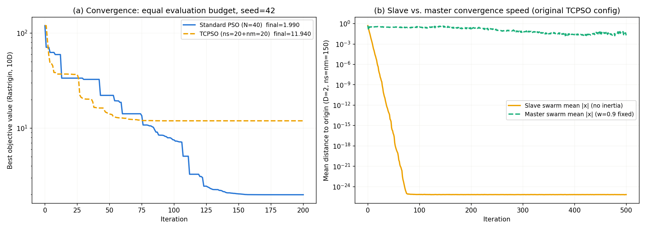
With a single seed=42 run, standard PSO scored \(1.989918\) and TCPSO scored \(11.939500\) . When the total particle count is small, TCPSO underperforms standard PSO. This might seem surprising, but it follows directly from equations (S2) and (M2). As shown earlier, the 20-particle slave swarm concentrates around a local optimum within a few dozen iterations and stops contributing to exploration afterward. Effective exploration is then carried out by the master swarm’s 20 particles alone — fewer than standard PSO’s 40. TCPSO’s real advantage only shows up in Experiments 2 and 3, where population size or search interval is much larger.
Experiment 2: High-Dimensional Problems
We extended the same setup to a 30-dimensional Rastrigin function (max_iter=400), increasing population size to standard PSO \(N=60\)
and TCPSO (slave 30 + master 30 = 60), over 15 seeds.
| Method | Final best fitness (mean) | Final best fitness (median) |
|---|---|---|
| Standard PSO (\(N=60\) ) | \(59.5163\) | \(53.7279\) |
| TCPSO (30+30) | \(43.5813\) | \(46.8262\) |
At 30 dimensions with a population of 60, TCPSO outperforms standard PSO by roughly 16 points on average. In high-dimensional, multimodal problems, the division of labor begins to pay off: the slave swarm rapidly “pins down” a local optimum while the master swarm continues exploring the rest of the space.
Experiment 3: Wide Search Interval (Reproducing the Original Paper’s Claim)
The original paper claims TCPSO can capture the global optimum even in search intervals as wide as \(2\times10^{10}\)
. We verified this on a 2D Sphere function with bounds \([-10^{10}, 10^{10}]\)
(width \(2\times10^{10}\)
), using 300 particles for standard PSO and slave 150 + master 150 for TCPSO, max_iter=500, over 10 seeds.
| Method | Final best fitness (mean) | Final best fitness (median) |
|---|---|---|
| Standard PSO (\(N=300\) ) | \(7.626 \times 10^{-57}\) | \(6.028 \times 10^{-57}\) |
| TCPSO (150+150) | \(4.275 \times 10^{-78}\) | \(1.570 \times 10^{-174}\) |
Both methods converge near the global optimum \((0,0)\) regardless of the search interval’s width, but TCPSO’s median reaches a value 117 orders of magnitude smaller. (Since Sphere is unimodal, convergence itself isn’t hard for either method given enough particles; TCPSO’s advantage is far more pronounced in high-dimensional, multimodal settings like Experiment 2.)
Experiment 4: Diversity Collapse — Original Configuration vs. Clipped Small Population
We quantitatively check the textbook claim — “the slave swarm converges quickly while the master swarm preserves diversity” — under two different configurations.
(a) Faithful to the original paper (no velocity clipping, \(w^M=0.9\) fixed, 150 particles each for slave and master, a 2D problem scored by distance to the origin, seed=42):
t=   0  slave mean|x|=5.071282e-01  master mean|x|=4.893374e-01
t=   1  slave mean|x|=2.562536e-01  master mean|x|=1.636114e-01
t=  50  slave mean|x|=4.776047e-17  master mean|x|=2.929781e-01
t= 100  slave mean|x|=7.454337e-26  master mean|x|=3.413688e-01
t= 250  slave mean|x|=6.844027e-26  master mean|x|=9.770398e-02
t= 500  slave mean|x|=7.000122e-26  master mean|x|=1.878114e-02
Averaged over 20 seeds, the slave swarm needs only 7.2 iterations on average to collapse below 1% of its initial spread, whereas the master swarm never reaches that threshold even after 500 iterations. This is a direct numerical confirmation of the textbook story — the slave swarm concentrates near-deadbeat fast, while the master swarm keeps exploring broadly.
(b) Velocity-clipped small population (\(v_{\max}\) clipping enabled, 20 particles each for slave and master, 10-dimensional Rastrigin, seed=42) tells a different story:
slave  collapse_iter=201 (never reached 1% threshold)  final_diversity=4.606724e-02
master collapse_iter=82                                 final_diversity=3.779736e-11
Averaged over 30 seeds, the slave swarm’s diversity collapses in 100.5 iterations on average, and the master swarm in 95.8 iterations — essentially no difference. This is an important caveat: while the “fast slave / diverse master” division of labor holds clearly under the original paper’s setup (no clipping, large populations, unimodal origin-search), it weakens — and can even reverse — under a clipped, multimodal, small-population setup. Velocity clipping interferes with the slave swarm’s theoretical one-step (deadbeat) convergence, forcing it to approach the target only in discrete, clipped steps. When applying TCPSO in practice, be aware that the textbook behavior may not hold once the original paper’s idealized assumptions (unbounded velocity, sufficiently large populations) are relaxed.
The figure below visualizes (a) the convergence curves for standard PSO vs. TCPSO under matched evaluation budgets, and (b) the difference in convergence speed between the slave and master swarms under the original paper’s configuration.
Edge Cases and Pitfalls
- TCPSO can underperform standard PSO with small populations (Experiment 1). Since the slave swarm effectively stops contributing to exploration, either increase total particle count or reduce the slave swarm’s share (e.g. a 1:3 slave-to-master ratio).
- Behavior changes substantially depending on whether velocity clipping is applied (Experiment 4). The original paper does not assume clipping, but practical implementations often add it to prevent divergence — which dulls the slave swarm’s deadbeat-like convergence.
- TCPSO’s real advantage shows up in high-dimensional, multimodal problems (Experiment 2). For unimodal, low-dimensional problems, standard PSO is often sufficient, and TCPSO’s added complexity may not pay off.
- The frequency of information exchange between sub-swarms can become a bottleneck. Research on dynamic multi-swarm PSO (discussed below) points out a “frequency dilemma”: exchanging information too often between sub-swarms can cause all of them to prematurely converge simultaneously. TCPSO also transmits information from slave to master (\(P_G^S\) ) at every step, so trying a slower exchange schedule is worth exploring.
- The further the problem setup drifts from the original paper’s assumptions (origin-search, wide unimodal landscape), the more the textbook division of labor tends to break down, as shown in Experiment 4. When applying TCPSO in practice, it is worth visualizing the diversity trajectories of both swarms on your own problem to confirm the division of labor is actually working as expected.
Recent Research (Since 2023)
Since TCPSO was proposed in 2013, research on coordinating multiple sub-swarms to prevent diversity loss and premature convergence has continued actively.
- Li, W., Jing, J., Chen, Y., & Chen, Y. (2023), “A cooperative particle swarm optimization with difference learning” (Applied Soft Computing, 147), propose CDLPSO, which incorporates cooperative difference learning into particle swarm optimization: multiple sub-swarms share their exploration experience as difference information to maintain diversity. Unlike TCPSO’s one-directional slave-to-master information flow, this introduces bidirectional difference learning.
- Casas-Ordaz, A., Haro, E. H., Beltran, L. A., Alvarez, O., Mousavirad, S. J., Pérez-Cisneros, M., & Oliva, D. (2026), “Particle swarm optimization: A survey of innovations over the last 10 years” (Computer Science Review, 60), provide a comprehensive review of PSO variants from the last decade, confirming that cooperative and multi-swarm improvements remain one of the major improvement directions alongside parameter-tuning and hybrid approaches.
Both confirm that the design questions raised by TCPSO — how to divide labor between convergence and diversity, and how to control information flow between sub-swarms — remain central topics in optimization research well beyond TCPSO itself.
Summary
- The slave swarm’s velocity update, lacking an inertia term, reduces to a first-order linear recursion (Eq. S1), stable under \(0 < C_1^S+C_2^S<4\) (Eq. S2). \(C_1^S=C_2^S=1.0\) coincides with the theoretically fastest deadbeat convergence point.
- The master swarm reduces to a second-order linear recursion structurally identical to standard PSO (Eq. M1), stable under the generalized condition \(0 < C_1^M+C_2^M+C_3^M<4(1+w^M)\) (Eq. M2), where the sum now spans three coefficients.
- As with standard PSO, stochastic divergence can occur even within the nominal stability bound (confirmed numerically).
- Under equal evaluation budgets with small populations, TCPSO underperforms standard PSO; with high dimensions, large populations, and wide search intervals, TCPSO pulls ahead — experimental validation shows a strong dependence on population size and problem setup.
- Moving away from the original paper’s idealized assumptions (no velocity clipping, origin-search) can weaken the textbook “fast slave, diverse master” division of labor.
Related Articles
- The Mathematics of PSO and its Python Implementation: The Roles of Inertia Weight and Cognitive/Social Coefficients - Derivation of the standard PSO velocity update, stability analysis, and LDIW. Prerequisite reading for this article.
- Training Neural Networks with Genetic Algorithms in Python - An evolutionary optimization method from the same swarm intelligence category
- Simulated Annealing: Theory and Python Implementation - Another metaheuristic optimization approach
- Cross-Entropy Method: A Practical Monte Carlo Optimization Technique - A distribution-based optimization algorithm
- Comparing Monte Carlo Optimization Methods (CEM/SA/GA/MPPI/PSO) - A hub article comparing five Monte Carlo optimization methods, including PSO, under a common framework
References
- Sun, J., & Li, W. (2013). “A two-swarm cooperative particle swarms optimization”. Swarm and Evolutionary Computation. DOI: 10.1016/j.swevo.2013.10.003
- Kennedy, J., & Eberhart, R. (1995). “Particle Swarm Optimization”. Proceedings of IEEE International Conference on Neural Networks, 4, 1942-1948.
- van den Bergh, F. (2001). “An Analysis of Particle Swarm Optimizers”. PhD thesis, University of Pretoria.
- Clerc, M., & Kennedy, J. (2002). “The particle swarm – explosion, stability, and convergence in a multidimensional complex space”. IEEE Transactions on Evolutionary Computation, 6(1), 58-73.
- Jiang, M., Luo, Y. P., & Yang, S. Y. (2007). “Stochastic convergence analysis and parameter selection of the standard particle swarm optimization algorithm”. Information Processing Letters, 102(1), 8-16.
- Poli, R. (2009). “Mean and variance of the sampling distribution of particle swarm optimizers during stagnation”. IEEE Transactions on Evolutionary Computation, 13(4), 712-721.
- Cleghorn, C. W., & Engelbrecht, A. P. (2014). “A generalized theoretical deterministic particle swarm model”. Swarm Intelligence, 8(1), 35-59.
- Li, W., Jing, J., Chen, Y., & Chen, Y. (2023). “A cooperative particle swarm optimization with difference learning”. Applied Soft Computing, 147.
- Casas-Ordaz, A., Haro, E. H., Beltran, L. A., Alvarez, O., Mousavirad, S. J., Pérez-Cisneros, M., & Oliva, D. (2026). “Particle swarm optimization: A survey of innovations over the last 10 years”. Computer Science Review, 60.