Bayesian Linear Regression: From Least Squares to Bayesian Estimation

Introduction

Regression is the task of learning the relationship between input data and corresponding output data, and predicting the output for unseen inputs. This article uses linear regression as an example to compare four representative parameter estimation methods: least squares, maximum likelihood estimation, MAP estimation, and Bayesian estimation, and explains their differences and characteristics.

Sections 1–3 trace the lineage of point estimates (least squares → MLE → MAP). Sections 4–6 derive the posterior and predictive distributions of Bayesian estimation with the full matrix algebra shown, not skipped. Section 4 in particular proves — rather than simply asserting — that “Gaussian MAP estimation equals ridge regression.” Finally, every formula is implemented in Python and checked numerically against scikit-learn, including an overfitting experiment with real measured numbers.

As the model, we consider a linear combination of basis functions \(\phi(x)\) , which are nonlinear functions of the input \(x\) . With \(w\) as the model parameters (weights) and \(\epsilon\) as the error, the model is:

Here, \(\Phi\) is the design matrix, where each row contains the basis function vector for a data point (\(\Phi \in \mathbb{R}^{N\times M}\) for \(N\) data points and \(M\) basis functions).

1. Least Squares Estimation

Least squares finds the parameters \(\hat{w}\) that minimize the sum of squared errors \(S(w)\) between the model predictions and the actual target values.

Setting the derivative of \(S(w)\) with respect to \(w\) to zero yields:

This has an analytical solution, making computation very fast. However, it is prone to overfitting when the training data is limited or the model has high degrees of freedom. It can also become numerically unstable when \(\Phi^T\Phi\) is singular or near-singular.

2. Maximum Likelihood Estimation (MLE)

MLE finds the parameters \(\hat{w}\) that maximize the probability of observing the data (likelihood).

Assuming the error term \(\epsilon\) follows a Gaussian distribution with mean \(0\) and variance \(\sigma^2\) , the conditional probability of the target \(y\) becomes a Gaussian with mean \(\Phi w\) and variance \(\sigma^2\) .

We maximize the log-likelihood:

Maximizing the log-likelihood is equivalent to minimizing the squared error term on the right. Therefore, under a Gaussian error assumption, MLE yields the same solution as least squares.

From here on we write the likelihood precision (inverse variance) as \(\beta = 1/\sigma^2\) .

3. MAP Estimation (Maximum A Posteriori)

MAP estimation is a general framework for suppressing overfitting. It treats the parameters \(w\) as random variables and introduces a prior distribution \(p(w)\) . Using Bayes’ theorem, it finds the \(\hat{w}\) that maximizes the posterior distribution \(p(w|y)\) .

Assuming a Gaussian prior with mean \(0\) and covariance \(\alpha^{-1}I\) for \(w\) , this encodes the prior belief that the weight values should be close to zero, acting as regularization that penalizes large weights.

The MAP estimate \(\hat{w}_{MAP}\) is (derived rigorously from the general formula in Section 4.2):

This has the same form as ridge regression (L2-regularized least squares), and the regularization term \(\frac{\alpha}{\beta}I\) ensures stable solutions even when \(\Phi^T\Phi\) is not invertible, while suppressing overfitting.

Note: the ratio is \(\alpha/\beta\) — “prior precision over likelihood precision” — not \(\beta/\alpha\) . Swapping numerator and denominator changes the regularization strength drastically (for \(\alpha=1,\beta=10\) , that’s a \(0.1\times\) vs. \(10\times\) difference — a factor of 100). Section 4.2 proves this correspondence explicitly.

4. Bayesian Estimation

Least squares, MLE, and MAP estimation all find a single optimal value for \(w\) (point estimation). However, this approach cannot express uncertainty about the parameters.

Bayesian estimation does not seek a single point estimate but instead computes the full posterior distribution \(p(w|y)\) , representing the probability distribution over all possible values of \(w\) given the observed data. A Gaussian prior combined with a Gaussian likelihood is conjugate, so the posterior is exactly Gaussian as well. Below we derive this explicitly with matrix algebra.

4.1 Deriving the posterior (full matrix algebra)

The MAP treatment above restricted the prior to the special form \(\mathcal{N}(0,\alpha^{-1}I)\) . Here we start from a general Gaussian prior with mean \(m_0\) and covariance \(S_0\) :

(setting \(m_0=0, S_0=\alpha^{-1}I\) recovers the Section 3 setup). The likelihood is

By Bayes’ theorem, \(p(w\mid y) \propto p(y\mid w)\, p(w)\) , so we add the exponents (negative log-densities) of the two Gaussians:

and collect terms in \(w\) . First expand each term:

Grouping the quadratic, linear, and constant terms in \(w\) :

If the posterior is Gaussian, \(\mathcal{N}(w\mid m_N, S_N)\) , its exponent has the form

(this expansion is called completing the square). Matching the quadratic and linear coefficients between the two expressions gives:

This is the closed-form posterior \(p(w\mid y) = \mathcal{N}(w\mid m_N, S_N)\) . It can be read as: the posterior precision-weighted mean is the sum of the prior “belief” (\(S_0^{-1}m_0\) ) and the data “evidence” (\(\beta\Phi^Ty\) ), each weighted by its own precision.

4.2 Regularization equivalence (proving the ridge-regression correspondence)

We now derive the MAP solution asserted in Section 3 rigorously from the general formula above. Substituting \(m_0=0\) , \(S_0=\alpha^{-1}I\) (a zero-mean, isotropic prior):

Factoring \(\beta\) out of the bracket, \(\alpha I + \beta \Phi^T\Phi = \beta\left(\Phi^T\Phi + \frac{\alpha}{\beta}I\right)\) , so

and \(\beta\) cancels completely. This is exactly the ridge-regression solution \(w_{ridge} = (\Phi^T\Phi + \lambda I)^{-1}\Phi^Ty\) with regularization strength \(\lambda = \alpha/\beta\) .

The same conclusion follows from directly minimizing the MAP objective. Maximizing the posterior is equivalent to minimizing \(E(w)\) , which under \(m_0=0,S_0=\alpha^{-1}I\) is

Differentiating with respect to \(w\) and setting to zero:

confirming \(\lambda=\alpha/\beta\) once both sides are divided by \(\beta\) . The equivalence “Gaussian-prior MAP = ridge regression” is proven by both routes — specializing the general posterior formula, and directly minimizing the objective — arriving at the same \(\lambda=\alpha/\beta\) . Section 5(b) verifies this equivalence numerically against sklearn.linear_model.Ridge.

4.3 Deriving the predictive distribution

For a new input \(x_*\) (basis vector \(\phi_* = \phi(x_*)\) ), prediction requires marginalizing over all possible \(w\) under the posterior \(p(w\mid y)=\mathcal{N}(w\mid m_N, S_N)\) . This is the predictive distribution:

This integral is exactly the marginal distribution of the linear transformation \(y_* = \phi_*^Tw + \epsilon_*\) of \(w\sim\mathcal{N}(m_N,S_N)\) , plus independent noise \(\epsilon_*\sim\mathcal{N}(0,\beta^{-1})\) . In general, if \(x\sim\mathcal{N}(\mu,\Lambda^{-1})\) and \(y\mid x\sim\mathcal{N}(Ax+b, L^{-1})\) , then the marginal of \(y\) is

(this is the standard Gaussian marginalization identity — Bishop, Pattern Recognition and Machine Learning, Eq. 2.115). Substituting \(A=\phi_*^T\) (a \(1\times M\) row vector), \(b=0\) , \(\Lambda^{-1}=S_N\) , \(L^{-1}=\beta^{-1}\) :

The predictive variance being a sum of two terms is the key structural fact here.

• \(\beta^{-1}\) : the variance of the observation noise itself — an irreducible error (aleatoric uncertainty) that never vanishes no matter how much data arrives.
• \(\phi_*^T S_N \phi_*\) : the term arising from posterior parameter uncertainty \(S_N\) (epistemic uncertainty). Since \(S_N^{-1}=S_0^{-1}+\beta\Phi^T\Phi\) grows monotonically as \(\Phi^T\Phi\) accumulates with more data, \(S_N\) itself shrinks monotonically. Hence as \(N\to\infty\) , \(\phi_*^TS_N\phi_*\to 0\) and the predictive variance asymptotes to the irreducible floor \(\beta^{-1}\) .

The magnitude of \(\phi_*^TS_N\phi_*\) also depends on the direction of \(\phi_*\) . In regions dense with training data, \(\Phi^T\Phi\) has large eigenvalues along that direction, so \(S_N\) is small there and uncertainty is suppressed. In regions with sparse or no training data (extrapolation), the corresponding eigenvalues stay small, so \(S_N\) remains large there — and this is further amplified by \(\phi_*\) itself (for a polynomial basis, \(\|\phi_*\|\) grows rapidly outside the training range). This is the mathematical basis for the intuition that “confidence intervals widen where there is no data.” Section 5 confirms this quantitatively with real N=8 vs. N=100 data.

5. Numerical Verification in Python

We now verify the derivations above by writing and running actual code. To match the existing experiments in Section 6, we use a 9th-degree polynomial basis, \(\phi_j(x)=x^j\ (j=0,\dots,9)\) .

import numpy as np
from numpy.linalg import inv
from sklearn.linear_model import BayesianRidge, Ridge

DEGREE = 9

def design_matrix(x):
    x = np.asarray(x).reshape(-1)
    return np.vstack([x**j for j in range(DEGREE + 1)]).T  # shape (N, 10)

def true_function(x):
    return np.sin(2 * np.pi * x)

def make_data(n, noise_std, seed):
    rng = np.random.RandomState(seed)
    x = np.sort(rng.uniform(0, 1, size=n))
    y = true_function(x) + rng.normal(0, noise_std, size=n)
    return x, y

def posterior(Phi, y, alpha, beta, m0=None, S0=None):
    """Direct implementation of the Section 4.1 formula:
       S_N^{-1} = S0^{-1} + beta * Phi^T Phi
       m_N = S_N (S0^{-1} m0 + beta * Phi^T y)"""
    M = Phi.shape[1]
    if S0 is None:
        S0 = np.eye(M) / alpha
    if m0 is None:
        m0 = np.zeros(M)
    S0_inv = inv(S0)
    S_N_inv = S0_inv + beta * Phi.T @ Phi
    S_N = inv(S_N_inv)
    m_N = S_N @ (S0_inv @ m0 + beta * Phi.T @ y)
    return m_N, S_N

def predictive(phi_star, m_N, S_N, beta):
    """Section 4.3 predictive distribution: mean and the two-term variance"""
    mean = phi_star @ m_N
    var = 1.0 / beta + phi_star @ S_N @ phi_star
    return mean, var

(a) Matching sklearn’s BayesianRidge

sklearn.linear_model.BayesianRidge estimates the noise precision and weight precision via type-II maximum likelihood (evidence maximization). If we plug those two estimated precisions directly into the Section 4.1 formula, the result should match sklearn’s own posterior mean coef_ and posterior covariance sigma_ (note sklearn’s naming is swapped relative to this article: its alpha_ is the noise precision — our \(\beta\) — and its lambda_ is the weight precision — our \(\alpha\) ).

N_CHECK, NOISE_STD = 30, 0.2
x_chk, y_chk = make_data(N_CHECK, NOISE_STD, seed=1)   # y = sin(2πx) + noise
Phi_chk = design_matrix(x_chk)

br = BayesianRidge(fit_intercept=False, tol=1e-10, max_iter=1000)
br.fit(Phi_chk, y_chk)
beta_hat, alpha_hat = br.alpha_, br.lambda_             # note the sklearn naming swap

m_N_scratch, S_N_scratch = posterior(Phi_chk, y_chk, alpha_hat, beta_hat)

print(np.max(np.abs(m_N_scratch - br.coef_)))    # max abs diff, posterior mean
print(np.max(np.abs(S_N_scratch - br.sigma_)))   # max abs diff, posterior covariance

Result:

sklearn estimated noise precision  (beta) : 38.033741
sklearn estimated weight precision (alpha): 0.008128
max |m_N(scratch) - coef_(sklearn)|        : 2.300e-11
max |S_N(scratch) - sigma_(sklearn)|       : 2.243e-10

The from-scratch posterior mean and covariance match sklearn’s to within ~\(10^{-10}\) — direct numerical confirmation that the Section 4.1 derivation is correct.

(b) Numerically verifying the ridge-regression equivalence

We check the \(\lambda=\alpha/\beta\) correspondence proven in Section 4.2 using fixed \(\alpha=1.0,\ \beta=10.0\) (the same values as the Section 6 experiment).

ALPHA_FIX, BETA_FIX = 1.0, 10.0
x15, y15 = make_data(15, 1.0 / np.sqrt(BETA_FIX), seed=2)
Phi15 = design_matrix(x15)

m_N_fix, S_N_fix = posterior(Phi15, y15, ALPHA_FIX, BETA_FIX)

lam = ALPHA_FIX / BETA_FIX  # = 0.1
ridge = Ridge(alpha=lam, fit_intercept=False, solver="cholesky").fit(Phi15, y15)
print(np.max(np.abs(m_N_fix - ridge.coef_)))

Result:

alpha=1.0, beta=10.0  =>  lambda = alpha/beta = 0.1
max |m_N - w_ridge|                         : 2.665e-15
(sanity check) using the WRONG ratio beta/alpha = 10.0: max diff = 1.600e+00  (large, as expected)

Using the correct ratio \(\lambda=\alpha/\beta=0.1\) , the coefficients match Ridge to double-precision rounding error (\(10^{-15}\) ), whereas using the swapped ratio \(\beta/\alpha=10\) produces coefficients off by as much as \(1.6\) . This confirms in practice just how much the numerator/denominator mix-up flagged in Section 3 would have mattered.

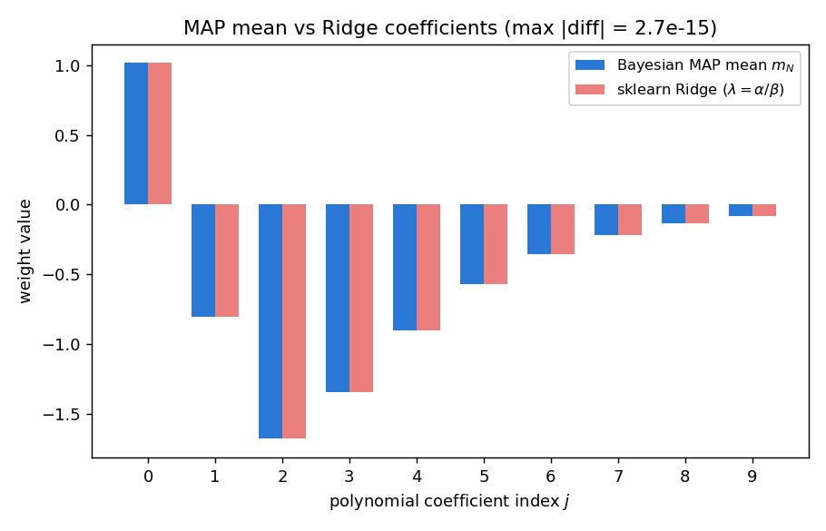
The figure below overlays \(m_N\) (blue) and the Ridge coefficients (red) for each of the 10 polynomial coefficients. The bars are essentially indistinguishable — the maximum difference, as noted in the title, is \(2.7\times10^{-15}\) .

(c) Overfitting and predictive-uncertainty shrinkage: N=8 vs. N=100

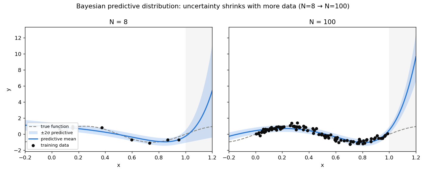
Section 4.3 argued that predictive variance shrinks as more data arrives. We now quantify this by comparing \(N=8\) (few points, prone to overfitting) against \(N=100\) (many points). Noise is \(\sigma=0.2\) (\(\beta=1/\sigma^2=25\) ), with the prior fixed at \(\alpha=1.0\) .

NOISE_STD, BETA_EXP, ALPHA_EXP = 0.2, 1.0 / 0.2**2, 1.0
x_interior, x_edge = 0.5, 1.1  # 0.5 = inside training range, 1.1 = outside [0,1] (extrapolation)

for n in (8, 100):
    x_n, y_n = make_data(n, NOISE_STD, seed=42)
    Phi_n = design_matrix(x_n)
    m_N_n, S_N_n = posterior(Phi_n, y_n, ALPHA_EXP, BETA_EXP)
    _, var_i = predictive(design_matrix([x_interior])[0], m_N_n, S_N_n, BETA_EXP)
    _, var_e = predictive(design_matrix([x_edge])[0], m_N_n, S_N_n, BETA_EXP)
    print(n, np.sqrt(var_i), np.sqrt(var_e))

Result:

N=  8: predictive std at x=0.5 (interior)      : 0.22929
N=  8: predictive std at x=1.1 (extrapolation) : 1.11805
N=100: predictive std at x=0.5 (interior)      : 0.20285
N=100: predictive std at x=1.1 (extrapolation) : 0.52754

shrinkage at x=0.5: 0.22929 / 0.20285 = 1.13x
shrinkage at x=1.1: 1.11805 / 0.52754 = 2.12x

irreducible noise floor sqrt(1/beta) = 0.20000
N=100 interior predictive std 0.20285 is essentially at this floor

Inside the training range (\(x=0.5\) ), even \(N=8\) already has nearby data points, so the difference in predictive std is a mild \(1.13\times\) . Outside the training range, at the extrapolation point (\(x=1.1\) ), the values are \(1.118\) (N=8) vs. \(0.528\) (N=100) — a \(2.12\times\) difference. Moreover, the N=100 interior predictive std of \(0.20285\) has essentially reached the theoretical irreducible-noise floor \(\sqrt{1/\beta}=0.2\) , consistent with the Section 4.3 claim that as \(N\to\infty\) the epistemic term vanishes and predictive variance asymptotes to \(\beta^{-1}\) .

The figure below overlays the predictive mean (solid blue line) and \(\pm2\sigma\) confidence band (blue shading), the true function (dashed gray), and the training data (black dots), for \(N=8\) (left) and \(N=100\) (right). The gray shaded region marks the area outside the training range \([0,1]\) (extrapolation). For \(N=8\) , the confidence band widens dramatically in the extrapolation region and the predictive mean diverges substantially from the true function; for \(N=100\) , the same extrapolation region shows a visibly narrower band.

6. Experimental Results (existing visualizations)

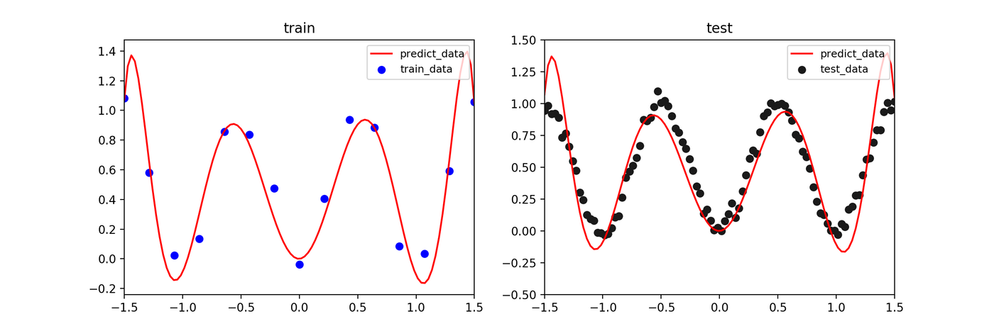
• Data: 15 training points generated from \(y = \sin(2\pi x)\) with added noise
• Basis functions: 9th-degree polynomial (\(f_j(x) = x^j, j=0, ..., 9\) )
• Hyperparameters: \(\alpha=1.0, \beta=10.0\) (same setup as the Section 5(b) numerical check)

Least Squares / Maximum Likelihood Estimation

The model tries to fit the training data closely, causing large oscillations in regions without data – a clear case of overfitting.

MAP Estimation

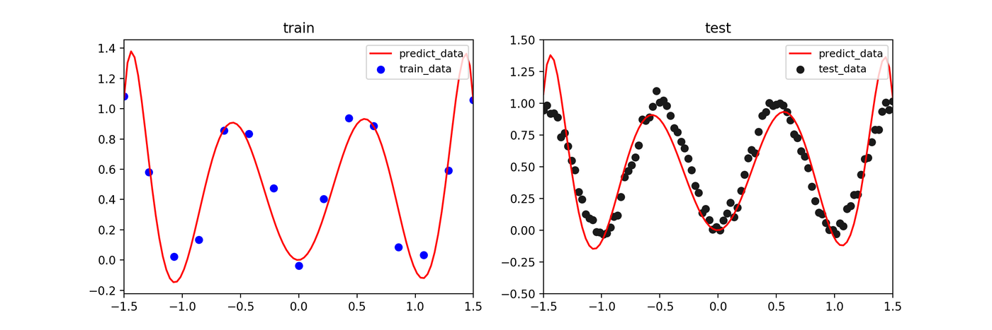
The prior distribution (regularization) suppresses overfitting, yielding a smoother prediction curve.

Bayesian Estimation

In addition to a smooth prediction (mean, solid line) similar to MAP, the prediction uncertainty increases in regions with less training data, as shown by the widening confidence interval (blue shaded area).

Model Evaluation (Coefficient of Determination \(R^2\) )

The coefficient of determination indicates how well the model fits the data (closer to 1 is better). MAP and Bayesian estimation (mean) achieve higher scores than least squares.

Effect of Hyperparameter \(\beta\)

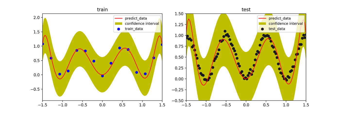
In Bayesian estimation, increasing the likelihood precision parameter \(\beta\) (inverse noise variance) causes the model to fit training data more tightly. When \(\beta\) is too large, the confidence interval narrows and the result approaches overfitting.

• \(\beta=50\)
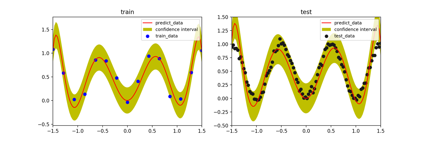
• \(\beta=100\)
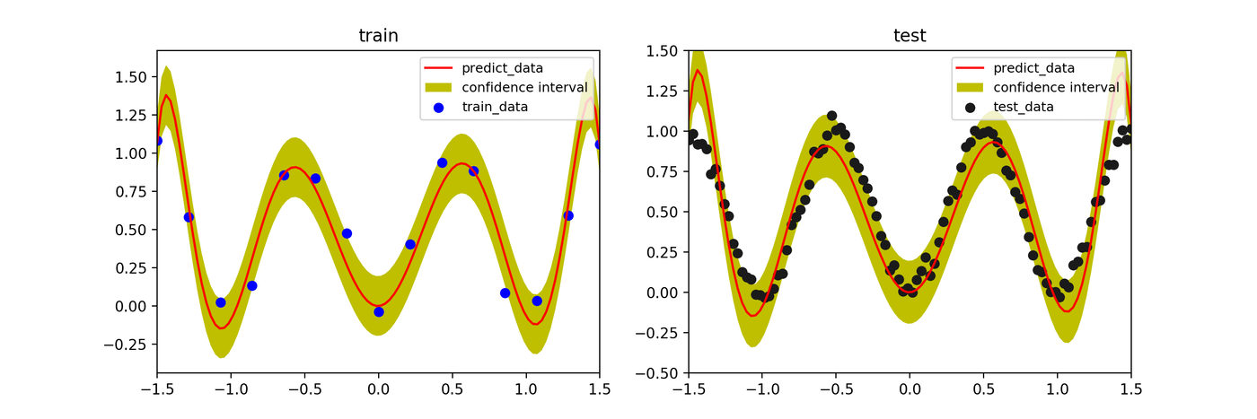
• \(\beta=1000\)

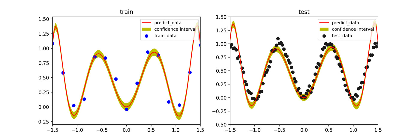
Summary

• Least Squares / MLE: Simple and fast, but prone to overfitting.
• MAP Estimation: Introduces a prior (regularization) to suppress overfitting. Gaussian-prior MAP estimation is exactly equivalent to ridge regression with \(\lambda=\alpha/\beta\) (proved in Section 4.2, verified numerically to \(10^{-15}\) precision in Section 5(b)).
• Bayesian Estimation: Keeps parameter uncertainty as the posterior covariance \(S_N\) , and separates the predictive variance \(\sigma_N^2(x_*)=\beta^{-1}+\phi_*^TS_N\phi_*\) into “irreducible noise” and “parameter uncertainty” terms. The latter shrinks as data accumulates, most dramatically outside the training range (measured shrinkage of 2.12x in the extrapolation experiment).

The Bayesian regression carried out here in parameter space generalizes, by pushing the basis functions to infinite dimension and placing a Gaussian-process prior directly on the function itself, to the function-space view. That perspective is covered in Gaussian Process Regression: Fundamentals and Python Implementation .

References

• C.M. Bishop, Pattern Recognition and Machine Learning , Springer (2006)
• Atsushi Suyama, Introduction to Machine Learning with Bayesian Inference , Kodansha (2017)