What is the Unscented Transformation?
The Unscented Transformation (UT) is a method for estimating the mean \(\bar{y}\) and covariance \(P_y\) of a random variable \(y = f(x)\) , where \(x\) is transformed by a nonlinear function \(f\) , given the known mean \(\bar{x}\) and covariance \(P_x\) of \(x\) .
One approach is to estimate these quantities using Monte Carlo sampling:
\[ \bar{y}\simeq\frac{1}{N}\sum_{i=1}^Nf(x_i) \] \[ P_y \simeq \frac{1}{N}\sum_{i=1}^N(f(x_i)-\bar{y})(f(x_i)-\bar{y})^T \]However, this requires a very large number of samples \(N\) for accurate estimation, making it computationally expensive.
The UT solves this problem by using a small set of carefully chosen representative points (sigma points) to efficiently and accurately estimate the statistical properties of the transformed variable – without any linear approximation. This retains the benefits of Monte Carlo methods (handling nonlinearity) while drastically reducing computational cost. In this article we prove why this particular set of sigma points and weights reproduces the mean and covariance exactly, and then verify the numbers by actually running the code.
Reference: What is UKF (Unscented Kalman Filter)?
Python Implementation
Here we consider transforming a 2-dimensional input \(X=(X_1, X_2)\) to a 1-dimensional output \(Y=f(X)=X_1 \cdot X_2\) .
1. Input Random Variable Setup
Define the mean vector \(\bar{x}\) and covariance matrix \(P_x\) of the input \(X\) .
\[ \bar{x} = [E[X_1], E[X_2]] \] \[ P_x = \begin{pmatrix} \text{Var}[X_1] & \text{Cov}[X_1, X_2] \\ \text{Cov}[X_2, X_1] & \text{Var}[X_2] \end{pmatrix} \]As an example, assume \(X_1\) has mean 0 and variance 1, and \(X_2\) has mean 1 and variance 4, with covariance 2.
import numpy as np
import scipy.linalg

# Dimension of input x
n = 2
# Dimension of output y
m = 1

# Mean vector and covariance matrix of x
x_mean = np.array([0.0, 1.0])
x_P = np.array([[1.0, 2.0], [2.0, 4.0]])

print(f"Input x mean: {x_mean}")
print(f"Input x covariance matrix:\n{x_P}")


# Nonlinear transformation f(x) = x[0] * x[1]
def f(x):
    return np.array([x[0] * x[1]])
Output:
Input x mean: [0. 1.]
Input x covariance matrix:
[[1. 2.]
 [2. 4.]]
Note that the correlation coefficient of this covariance matrix is \(\rho = \mathrm{Cov}(X_1,X_2)/\sqrt{\mathrm{Var}[X_1]\mathrm{Var}[X_2]} = 2/(1\cdot 2) = 1\) – i.e. \(X_1\) and \(X_2\) are perfectly (linearly) dependent, a degenerate case. As we will see below, this is a special case that requires care when computing the matrix square root.
2. Sigma Point Calculation
Sigma points are carefully chosen representative points that accurately capture the mean and covariance of the input random variable \(x\) . They are computed using the following formulas:
\[ \sigma_0 = \bar{x} \tag{1} \] \[ \sigma_i = \bar{x} + \left(\sqrt{(n+\lambda) P_x}\right)_i, \quad i=1, \dots, n \tag{2} \] \[ \sigma_i = \bar{x} - \left(\sqrt{(n+\lambda) P_x}\right)_i, \quad i=n+1, \dots, 2n \tag{3} \]Here, \(\left(\sqrt{(n+\lambda)P_x}\right)_i\) represents the \(i\) -th column of the matrix square root (e.g., via Cholesky decomposition).
The parameter \(\lambda\) is calculated as:
\[ \lambda = \alpha^2 (n + \kappa) - n \tag{4} \]- \(\alpha\) : A scalar that determines the spread of sigma points around the mean (typically a small positive value between 0 and 1).
- \(\kappa\) : A tuning parameter, usually set to 0.
Why these weights reproduce the mean and covariance exactly (proof)
Rather than accepting the sigma points of Eq. (1)-(3) and the weights of Eq. (6)(7) below at face value, let’s prove why this particular set of \(2n+1\) points and weights reproduces the input mean \(\bar x\) and covariance \(P_x\) exactly, for any probability distribution (not just Gaussian).
Let \(S=\sqrt{(n+\lambda)P_x}\) be a matrix square root (\(SS^T=(n+\lambda)P_x\) ) with \(i\) -th column \(s_i\) . Then Eq. (2)(3) can be rewritten as \(\sigma_i=\bar x + s_i\) (\(i=1,\dots,n\) ) and \(\sigma_{i+n}=\bar x - s_i\) (\(i=1,\dots,n\) ).
(a) The weights sum to 1
\[ \sum_{i=0}^{2n} w_i = \frac{\lambda}{n+\lambda} + 2n \cdot \frac{1}{2(n+\lambda)} = \frac{\lambda+n}{n+\lambda} = 1 \](b) The mean is reproduced exactly
\[ \sum_{i=0}^{2n} w_i \sigma_i = w_0\bar x + \sum_{i=1}^n \frac{1}{2(n+\lambda)}(\bar x+s_i) + \sum_{i=1}^n \frac{1}{2(n+\lambda)}(\bar x-s_i) \]The \(+s_i\) and \(-s_i\) terms cancel, leaving
\[ \sum_{i=0}^{2n} w_i \sigma_i = \left(w_0+\frac{n}{n+\lambda}\right)\bar x = \left(\frac{\lambda}{n+\lambda}+\frac{n}{n+\lambda}\right)\bar x = \bar x \]Because the sigma points are placed symmetrically (\(+s_i\) and \(-s_i\) ) around the mean, the weighted mean is exactly \(\bar x\) regardless of the value of \(\lambda\) or the content of \(P_x\) .
(c) The covariance is reproduced exactly
Since \(\sigma_0-\bar x=0\) , the \(w_0\) term contributes nothing, so
\[ \sum_{i=0}^{2n} w_i(\sigma_i-\bar x)(\sigma_i-\bar x)^T = \frac{1}{2(n+\lambda)}\sum_{i=1}^n \left[s_is_i^T + (-s_i)(-s_i)^T\right] = \frac{1}{n+\lambda}\sum_{i=1}^n s_is_i^T \]By the definition of matrix multiplication, \(\sum_{i=1}^n s_is_i^T = SS^T\) , so
\[ \sum_{i=0}^{2n} w_i(\sigma_i-\bar x)(\sigma_i-\bar x)^T = \frac{SS^T}{n+\lambda} = \frac{(n+\lambda)P_x}{n+\lambda} = P_x \]From (a)-(c), as long as \(n+\lambda \neq 0\) , the sigma-point set reproduces the first two moments (mean and covariance) of the input distribution exactly, for any distribution – no Gaussian assumption is used anywhere in the proof. Sigma points are not “sample points that approximate a distribution”; they are, by construction, “a discrete distribution consisting of exactly \(2n+1\) atoms that has the specified mean and covariance.” ( Fundamentals of Filtering Methods in Signal Processing gives only an intuitive scalar-variable Taylor-expansion argument for why UKF is accurate to second order; here we give the rigorous proof for general dimension \(n\) .)
Why the post-transformation mean is accurate to second order
Let’s also see why the output \(y=f(x)\) (scalar output here) is accurate up to the second-order Taylor term. Expanding \(f\) around \(\bar x\) :
\[ f(x) = f(\bar x) + \nabla f(\bar x)^T(x-\bar x) + \frac{1}{2}(x-\bar x)^T H(x-\bar x) + R_3(x) \](\(H\) is the Hessian of \(f\) , \(R_3\) is the third-and-higher-order remainder). Taking the sigma-point weighted average, the first-order term vanishes by (b) since \(\sum_i w_i(\sigma_i-\bar x)=0\) , and the second-order term matches \(\frac{1}{2}\mathrm{tr}(HP_x)\) exactly by (c):
\[ \sum_{i=0}^{2n} w_i f(\sigma_i) = f(\bar x) + \frac{1}{2}\mathrm{tr}(HP_x) + \sum_{i=0}^{2n} w_i R_3(\sigma_i) \]Meanwhile, the true expectation is obtained by simply taking the expectation of the same Taylor expansion over the random variable \(X\) :
\[ E[f(X)] = f(\bar x) + \frac{1}{2}\mathrm{tr}(HP_x) + E[R_3(X)] \]The two only differ in the third-and-higher-order remainder terms. In particular, when \(f\) is a quadratic polynomial (such as \(f(x)=x_1x_2\) in this article), \(R_3\equiv0\) identically, so the sigma-point mean estimate exactly matches the true mean regardless of the shape of the input distribution. EKF, by contrast, linearizes \(f\) using only the Jacobian and therefore captures only the first-order term, completely missing this second-order bias term \(\frac{1}{2}\mathrm{tr}(HP_x)\) (EKF’s propagated mean is simply \(f(\bar x)\) ). We verify this difference numerically below.
Implementation pitfall: matrix square roots of a singular covariance matrix
The square root \(\sqrt{(n+\lambda)P_x}\) in Eq. (2)(3) is usually computed via Cholesky decomposition. However, as noted above, \(P_x=\begin{pmatrix}1&2\\2&4\end{pmatrix}\) in this article is a singular matrix with correlation 1 (\(\det P_x=0\) , eigenvalues \(\{0,5\}\) ). Cholesky decomposition, which requires positive-definiteness, fails on such a matrix.
try:
    scipy.linalg.cholesky(x_P, lower=True)
except Exception as e:
    print(f"cholesky failed: {type(e).__name__}: {e}")
Output:
cholesky failed: LinAlgError: Internal potrf return info = [2] for slices [0].
When the covariance matrix is singular (or only marginally positive semidefinite due to numerical error), a Cholesky-based implementation simply crashes. This isn’t limited to the extreme case of perfect correlation – rank-deficient process noise or accumulated rounding error after long-horizon propagation can trigger the same failure. In practice you need a robust square root that does not require strict positive-definiteness. An eigenvalue decomposition works for any positive semidefinite matrix (eigenvalues \(\geq 0\) ):
def sym_sqrt(P):
    """Matrix square root of a symmetric PSD matrix via eigendecomposition (works even for singular matrices)"""
    eigvals, eigvecs = np.linalg.eigh(P)
    eigvals = np.clip(eigvals, 0, None)  # clip tiny negative eigenvalues from numerical error
    return eigvecs @ np.diag(np.sqrt(eigvals)) @ eigvecs.T


S_check = sym_sqrt(x_P)
print(f"S_check @ S_check.T:\n{S_check @ S_check.T}")
Output:
S_check @ S_check.T:
[[1. 2.]
 [2. 4.]]
\(SS^T\)
exactly reproduces the original \(P_x\)
to machine precision. We use this sym_sqrt for the rest of the sigma-point calculations.
3. Transformation and Statistical Calculation
Each sigma point is transformed by the nonlinear function \(f\) to obtain \(y_{\sigma}\) :
\[ y_{\sigma,i} = f(\sigma_i) \tag{5} \]Next, the weights \(w_i\) for each sigma point are calculated:
\[ w_0 = \frac{\lambda}{n + \lambda} \tag{6} \] \[ w_i = \frac{1}{2(n + \lambda)} \quad \text{for } i=1, \dots, 2n \tag{7} \]Finally, the mean \(\bar{y}\) and covariance \(P_y\) of \(y\) are computed using these weights and transformed sigma points:
\[ \bar{y} \approx \sum_{i=0}^{2n} w_i y_{\sigma,i} \tag{8} \] \[ P_y \approx \sum_{i=0}^{2n} w_i (y_{\sigma,i} - \bar{y})(y_{\sigma,i} - \bar{y})^T \tag{9} \]We use Julier’s classic recommendation \(\kappa = 3-n\) (\(\kappa=1\) for \(n=2\) ) with \(\alpha=1\) (we examine below, in the “pitfall” section, exactly why the original \(\alpha=0.5,\kappa=0\) combination is problematic).
alpha = 1.0
kappa = 1.0  # Julier's classic recommendation kappa = 3 - n (kappa=1 for n=2)

# Eq. 4: Calculate lambda
lam = alpha**2 * (n + kappa) - n
print(f"lambda: {lam}, n+lambda: {n + lam}")

# Array to store sigma points (2n+1 sigma points)
sigma_points = np.zeros((n, 2 * n + 1))
# Eq. 1: First sigma point is the mean
sigma_points[:, 0] = x_mean
# Matrix square root of (n+lambda) * Px, via the eigendecomposition-based sym_sqrt
sqrt_term = sym_sqrt((n + lam) * x_P)
# Eq. 2, 3: Compute remaining sigma points
for i in range(n):
    sigma_points[:, i + 1] = x_mean + sqrt_term[:, i]
    sigma_points[:, i + n + 1] = x_mean - sqrt_term[:, i]

for i in range(2 * n + 1):
    print(f"  sigma_{i}: {sigma_points[:, i]}")

# Array to store weights
w = np.zeros(2 * n + 1)
# Eq. 6, 7: Weight calculation
w[0] = lam / (n + lam)
w[1:] = 1 / (2 * (n + lam))
print(f"\nweights: {w}, sum: {w.sum()}")

# Array to store transformed sigma points
sigma_y = np.zeros((m, 2 * n + 1))
# Eq. 5: Nonlinear transformation
for i in range(2 * n + 1):
    sigma_y[:, i] = f(sigma_points[:, i])

# Eq. 8: Calculate mean of y
y_mean = np.sum(w * sigma_y, axis=1)

# Eq. 9: Calculate covariance of y
y_P = np.zeros((m, m))
for i in range(2 * n + 1):
    diff = sigma_y[:, i] - y_mean
    y_P += w[i] * np.outer(diff, diff)  # Use outer product for (m,m) matrix

print(f"\nEstimated mean of output y: {y_mean}")
print(f"Estimated covariance matrix of output y:\n{y_P}")
Output:
lambda: 1.0, n+lambda: 3.0
  sigma_0: [0. 1.]
  sigma_1: [0.774597 2.549193]
  sigma_2: [1.549193 4.098387]
  sigma_3: [-0.774597 -0.549193]
  sigma_4: [-1.549193 -2.098387]

weights: [0.33333333 0.16666667 0.16666667 0.16666667 0.16666667], sum: 1.0

Estimated mean of output y: [2.]
Estimated covariance matrix of output y:
[[5.16]]
Let’s confirm that proof (a)-(c) actually holds by reconstructing the input mean and covariance from the sigma points:
recon_mean = np.sum(w * sigma_points, axis=1)
recon_P = np.zeros((n, n))
for i in range(2 * n + 1):
    diff = sigma_points[:, i] - recon_mean
    recon_P += w[i] * np.outer(diff, diff)

print(f"Reconstructed mean: {recon_mean} (matches: {np.allclose(recon_mean, x_mean)})")
print(f"Reconstructed covariance:\n{recon_P}\n(matches: {np.allclose(recon_P, x_P)})")
Output:
Reconstructed mean: [0. 1.] (matches: True)
Reconstructed covariance:
[[1. 2.]
 [2. 4.]]
(matches: True)
As the proof predicts, the mean and covariance reconstructed from the sigma points match \(\bar x\) , \(P_x\) to machine precision.
4. Numerical Verification: Analytic Solution vs. Monte Carlo
If \(X=(X_1,X_2)\) follows a Gaussian distribution \(\mathcal N(\bar x, P_x)\) , the mean and variance of \(Y=X_1X_2\) can be computed analytically using Wick’s theorem (Isserlis’ theorem). Writing \(X_1=\mu_1+\varepsilon_1\) , \(X_2=\mu_2+\varepsilon_2\) (where \(\varepsilon\) is zero-mean Gaussian with covariance \(\Sigma\) ):
\[ E[Y] = \mu_1\mu_2 + \Sigma_{12} \] \[ \mathrm{Var}[Y] = \mu_1^2\Sigma_{22} + \mu_2^2\Sigma_{11} + \Sigma_{11}\Sigma_{22} + \Sigma_{12}^2 + 2\mu_1\mu_2\Sigma_{12} \](The variance formula follows from Isserlis’ fourth-moment identity \(E[\varepsilon_1^2\varepsilon_2^2]=\Sigma_{11}\Sigma_{22}+2\Sigma_{12}^2\) and the fact that odd-order central moments of a Gaussian vanish identically.) Let’s substitute our numerical example and verify:
mu1, mu2 = x_mean
S11, S22, S12 = x_P[0, 0], x_P[1, 1], x_P[0, 1]
true_mean = mu1 * mu2 + S12
true_var = mu1**2 * S22 + mu2**2 * S11 + S11 * S22 + S12**2 + 2 * mu1 * mu2 * S12
print(f"Analytic: true_mean = {true_mean}, true_var = {true_var}")

rng = np.random.default_rng(0)
N = 2_000_000
# x_P is singular, so use method="eigh" (eigendecomposition-based sampling)
samples = rng.multivariate_normal(x_mean, x_P, size=N, method="eigh")
y_samples = samples[:, 0] * samples[:, 1]
print(f"Monte Carlo (N={N}): mean={y_samples.mean():.4f}, var={y_samples.var():.4f}")
Output:
Analytic: true_mean = 2.0, true_var = 9.0
Monte Carlo (N=2000000): mean=2.0010, var=9.0168
| Method | Mean \(E[Y]\) | Variance \(\mathrm{Var}[Y]\) |
|---|---|---|
| UT (\(\alpha=1,\kappa=1\) ) | 2.0 | 5.16 |
| Analytic (Gaussian assumption) | 2.0 | 9.0 |
| Monte Carlo (\(N=2\times10^6\) ) | 2.0010 | 9.0168 |
| EKF-equivalent (linearization only, \(f(\bar x)\) ) | 0.0 | ― |
As the proof predicts, UT’s mean estimate of 2.0 exactly matches the analytic solution and Monte Carlo, in stark contrast to the EKF-equivalent value of 0.0 (because \(f\) is quadratic, the third-and-higher-order remainder \(R_3\) from the proof vanishes identically). On the other hand, UT’s variance estimate of 5.16 underestimates the true value of 9.0 by roughly 43%. This is because \(\mathrm{Var}[Y]\) depends on the fourth moment of \(X\) (the \(\Sigma_{11}\Sigma_{22}+\Sigma_{12}^2\) term), whereas proof (a)-(c) only guarantees exact reproduction of the input’s first two moments (mean and covariance). Since \(2n+1\) sigma points generally cannot reproduce fourth moments, the accuracy of the variance estimate remains an approximation that depends on the choice of scaling parameter \(\lambda\) (i.e., \(\alpha,\kappa\) ).
Confirming that only the mean is distribution-independent
As the proof shows, the exactness of the mean for a quadratic \(f\) should hold regardless of the shape of the distribution (Gaussian or not). Let’s confirm this with a degenerate two-point distribution that has the same mean and covariance as \(X_1,X_2\) but is not Gaussian (\(P_x\) is singular, so placing two points along the nonzero eigenvector direction exactly reproduces the same mean and covariance):
eigvals, eigvecs = np.linalg.eigh(x_P)
idx = np.argmax(eigvals)
direction = eigvecs[:, idx]
scale = np.sqrt(eigvals[idx])

pts = np.array([x_mean + scale * direction, x_mean - scale * direction])
probs = np.array([0.5, 0.5])

disc_mean = (probs[:, None] * pts).sum(axis=0)
diffs = pts - disc_mean
disc_cov = sum(p * np.outer(d, d) for p, d in zip(probs, diffs))
y_disc = pts[:, 0] * pts[:, 1]
disc_y_mean = (probs * y_disc).sum()
disc_y_var = (probs * (y_disc - disc_y_mean) ** 2).sum()

print(f"Two-point distribution mean: {disc_mean} (matches: {np.allclose(disc_mean, x_mean)})")
print(f"Two-point distribution covariance:\n{disc_cov}\n(matches: {np.allclose(disc_cov, x_P)})")
print(f"Two-point distribution E[Y]={disc_y_mean}, Var[Y]={disc_y_var}")
Output:
Two-point distribution mean: [0. 1.] (matches: True)
Two-point distribution covariance:
[[1. 2.]
 [2. 4.]]
(matches: True)
Two-point distribution E[Y]=2.0, Var[Y]=1.0
Despite having exactly the same mean and covariance (\(\bar x=[0,1]\) , \(P_x=\begin{pmatrix}1&2\\2&4\end{pmatrix}\) ), this two-point distribution gives \(\mathrm{Var}[Y]=1.0\) , wildly different from the Gaussian case’s 9.0. Yet \(E[Y]\) agrees exactly at 2.0 in both cases. This is precisely what the proof predicts: the expectation of a quadratic \(f\) is uniquely determined by the input’s mean and covariance alone, but the variance (which involves fourth moments) depends on the shape of the distribution – no matter how carefully UT places its sigma points, it cannot obtain an exact variance without information about the fourth-and-higher moments of the input distribution.
5. Figure: Sigma Point Placement and the Post-Transformation Distribution
The previous example is degenerate (\(P_x\) singular, correlation 1) and collapses onto a single line in the 2D plane, which is not ideal for visualization. Here we visualize sigma-point placement and the post-transformation distribution using a non-singular covariance matrix instead.
x_P2 = np.array([[1.0, 1.5], [1.5, 4.0]])
print(f"det(P_x2) = {np.linalg.det(x_P2):.4f}, eigvals = {np.linalg.eigvalsh(x_P2)}")

sqrt_term2 = sym_sqrt((n + lam) * x_P2)
sigma_points2 = np.zeros((n, 2 * n + 1))
sigma_points2[:, 0] = x_mean
for i in range(n):
    sigma_points2[:, i + 1] = x_mean + sqrt_term2[:, i]
    sigma_points2[:, i + n + 1] = x_mean - sqrt_term2[:, i]

sigma_y2 = np.zeros((m, 2 * n + 1))
for i in range(2 * n + 1):
    sigma_y2[:, i] = f(sigma_points2[:, i])

y_mean2 = np.sum(w * sigma_y2, axis=1)
y_P2 = np.zeros((m, m))
for i in range(2 * n + 1):
    diff = sigma_y2[:, i] - y_mean2
    y_P2 += w[i] * np.outer(diff, diff)

S11b, S22b, S12b = x_P2[0, 0], x_P2[1, 1], x_P2[0, 1]
true_mean2 = mu1 * mu2 + S12b
true_var2 = mu1**2 * S22b + mu2**2 * S11b + S11b * S22b + S12b**2 + 2 * mu1 * mu2 * S12b

samples2 = rng.multivariate_normal(x_mean, x_P2, size=N)
y_samples2 = samples2[:, 0] * samples2[:, 1]

print(f"UT: y_mean2={y_mean2}, y_P2={y_P2}")
print(f"Analytic: true_mean2={true_mean2}, true_var2={true_var2}")
print(f"Monte Carlo: mean={y_samples2.mean():.4f}, var={y_samples2.var():.4f}")
Output:
det(P_x2) = 1.7500, eigvals = [0.378682 4.621318]
UT: y_mean2=[1.5], y_P2=[[2.644608]]
Analytic: true_mean2=1.5, true_var2=7.25
Monte Carlo: mean=1.5015, var=7.2674
Once again, UT’s mean estimate of 1.5 exactly matches the analytic solution and Monte Carlo, while its variance estimate of 2.64 substantially underestimates the true value of 7.25. The figure below visualizes the placement of the 5 sigma points for this non-singular example (left) and the post-transformation output distribution (right), using a separately generated set of \(N=20{,}000\) Monte Carlo samples for visualization only.
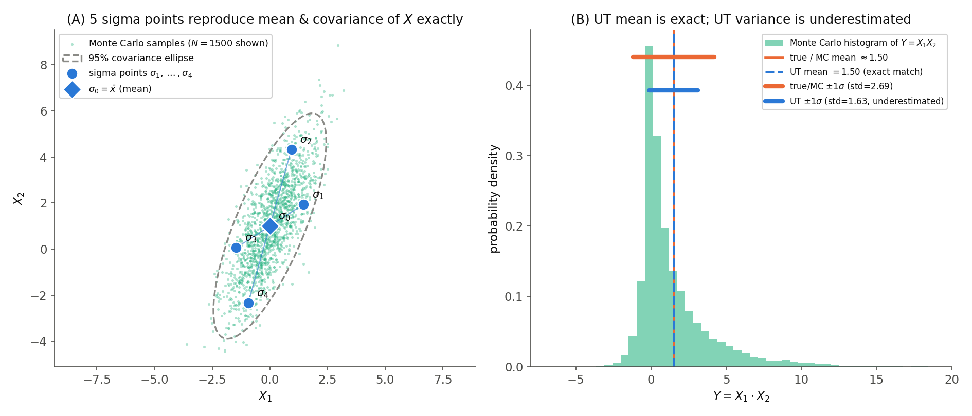
In the left panel, just 5 sigma points (blue circles/diamond) represent the 95% covariance ellipse (dashed gray) spanned by 1,500 of the 20,000 Monte Carlo samples plotted (green points) remarkably well. In the right panel, the histogram of the transformed output \(Y=X_1X_2\) (green) shows UT’s mean estimate (blue dashed line) exactly overlapping the true mean (orange solid line), while UT’s \(\pm1\sigma\) band (blue) is visibly narrower than the true \(\pm1\sigma\) band (orange) – a direct visual confirmation of the variance underestimation.
Pitfall: Negative Weights and Invalid Covariance Estimates
Looking at Eq. (6), when \(\lambda<0\) the central sigma point’s weight \(w_0\) can become negative. In fact, the original article’s parameter choice of \(\alpha=0.5,\kappa=0\) falls into exactly this trap.
alpha_bad, kappa_bad = 0.5, 0.0
lam_bad = alpha_bad**2 * (n + kappa_bad) - n
w_bad = np.zeros(2 * n + 1)
w_bad[0] = lam_bad / (n + lam_bad)
w_bad[1:] = 1 / (2 * (n + lam_bad))

sqrt_term_bad = sym_sqrt((n + lam_bad) * x_P)
sigma_points_bad = np.zeros((n, 2 * n + 1))
sigma_points_bad[:, 0] = x_mean
for i in range(n):
    sigma_points_bad[:, i + 1] = x_mean + sqrt_term_bad[:, i]
    sigma_points_bad[:, i + n + 1] = x_mean - sqrt_term_bad[:, i]

sigma_y_bad = np.zeros((m, 2 * n + 1))
for i in range(2 * n + 1):
    sigma_y_bad[:, i] = f(sigma_points_bad[:, i])

y_mean_bad = np.sum(w_bad * sigma_y_bad, axis=1)
y_P_bad = np.zeros((m, m))
for i in range(2 * n + 1):
    diff = sigma_y_bad[:, i] - y_mean_bad
    y_P_bad += w_bad[i] * np.outer(diff, diff)

print(f"lambda_bad: {lam_bad}, n+lambda_bad: {n + lam_bad}")
print(f"weights_bad: {w_bad}, sum: {w_bad.sum()}")
print(f"y_mean_bad: {y_mean_bad}, y_P_bad: {y_P_bad}")
Output:
lambda_bad: -1.5, n+lambda_bad: 0.5
weights_bad: [-3.  1.  1.  1.  1.], sum: 1.0
y_mean_bad: [2.], y_P_bad: [[-1.64]]
The mean estimate is still correctly 2.0, as the proof guarantees, but the covariance estimate becomes -1.64, a negative value. Since variance can never be negative, this is clearly an invalid estimate. The cause lies in the fact that covariance is computed as a weighted sum of rank-1 outer products \((y_{\sigma,i}-\bar y)(y_{\sigma,i}-\bar y)^T\) (Eq. 9): the central sigma point’s weight \(w_0=-3\) is large and negative, and it more than cancels out the positive contributions from the other four points, flipping the total to negative.
This problem grows worse as the dimension \(n\) increases – as we prove in detail in Cubature Kalman Filter (CKF): Theory and Python Implementation , UKF using Julier’s classic recommendation \(\kappa=3-n\) is guaranteed to produce a negative \(w_0\) for \(n>9\) . Practical mitigations include:
- keeping \(\alpha\) close to 1 (so \(\lambda\) doesn’t become excessively negative), or
- adopting van der Merwe scaling (used in Unscented Kalman Filter (UKF): Theory and Python Implementation ), which uses separate weights for the mean and covariance, \(w_0^{(c)}=\lambda/(n+\lambda)+(1-\alpha^2+\beta)\) .
Either way, the key implementation takeaway is that UT weights should always be validated – blindly applying Eq. (6)(7) can yield an invalid covariance estimate.
Recent Research Trends
Research continues on the very issue behind the pitfall above: UT’s weighting scheme is a fixed formula that implicitly assumes a particular distributional shape (typically Gaussian). Majewski, Modzelewski, Żugaj, & Lichota (2026), “Robust Unscented Kalman Filtering via Recurrent Meta-Adaptation of Sigma-Point Weights” ( arXiv:2603.04360 ), propose the Meta-Adaptive UKF (MA-UKF), which reformulates sigma-point weight synthesis as a hyperparameter-optimization problem rather than relying on a fixed scaling-parameter formula. A recurrent context encoder compresses the history of measurement innovations into a compact latent embedding, which drives a policy network that dynamically generates sigma-point weights at each time step, improving robustness to heavy-tailed measurement noise and unseen dynamic regimes. This is a data-driven attempt to address exactly the limitation demonstrated in this article – that fixed-formula weights can yield inaccurate (or even invalid) covariance estimates when the distribution deviates from the assumptions baked into the formula.
UT also continues to be used well beyond target tracking and Kalman filtering, as a general-purpose uncertainty-propagation tool. Chu, Shrestha, Gu, & Gross (2025), “Robust Flower Cluster Matching Using The Unscented Transform” ( arXiv:2503.20631 ), use the UT to efficiently estimate the spatial uncertainty tolerance of plant descriptors when an agricultural robot tracks flower clusters with an RGB-D camera, enabling robust image registration despite visual changes and occlusion over time. This is a 2025 example of the UT’s core property – proven in this article – that a small number of points can accurately propagate mean and covariance through a nonlinear transformation, still being put to practical use in robotics and agricultural vision applications.
Where This Article Fits (avoiding overlap with related articles)
Several articles on this blog touch on the Unscented Transformation and sigma points; here is how they divide the work:
- Fundamentals of Filtering Methods in Signal Processing – gives only an intuitive, scalar-variable explanation (via Taylor expansion) of why UKF captures the second-order term, and defers the rigorous multivariate proof to this article.
- This article – proves, for general dimension \(n\) , that the sigma-point/weight set reproduces the input’s mean and covariance (first two moments) exactly, and derives via Taylor expansion why the post-transformation mean is accurate to second order. It also covers numerical verification, figures, pitfalls, and recent research trends.
- Cubature Kalman Filter (CKF): Theory and Python Implementation – proves that the spherical cubature rule is exact up to third-degree polynomials, a different (higher) degree of exactness than this article’s “exact up to second moment” result, and quantitatively examines the weight-stability differences (the negative-weight problem) between UKF and CKF.
- Unscented Kalman Filter (UKF): Theory and Python Implementation – builds on the proofs in this article and the CKF article, focusing instead on the Kalman-filter implementation (predict/update steps) and accuracy comparison against EKF.
This implementation demonstrates how the mean and covariance of a nonlinearly transformed random variable can be efficiently estimated from a small number of sigma points. The Unscented Transformation is the foundation of the Unscented Kalman Filter (UKF).
Related Articles
- Particle Filter Python Implementation: Comparing Resampling Methods - A Monte Carlo-based nonlinear filtering approach that represents distributions using many weighted particles instead of sigma points.
- Cubature Kalman Filter (CKF): Theory and Python Implementation - Addresses sigma point selection issues in UT by using cubature points derived from spherical-radial cubature rules.