Creating a Neural Network Class
import torch
import torch.nn as nn
import torch.nn.functional as F
import torch.optim as optim
import numpy as np
Modern PyTorch tensors support automatic differentiation (autograd) natively, so wrapping them in torch.autograd.Variable is unnecessary (since PyTorch 0.4, Variable and Tensor have been merged; Variable survives only as a deprecated alias).
Inherit from nn.Module to define the neural network (NN) architecture, optimizer, and loss function. The optimizer adjusts the neural network parameters to minimize the loss computed by the loss function.
- Optimizer variants: From SGD to Adam: Evolution of Gradient-Based Optimization
class Model(nn.Module):
    def __init__(self, input_dim, output_dim):
        super(Model, self).__init__()
        # NN layers
        self.fc1 = nn.Linear(input_dim, 100)
        self.fc2 = nn.Linear(100, 100)
        self.fc3 = nn.Linear(100, output_dim)
        # Learning rate and parameter update method
        self.optimizer = optim.SGD(self.parameters(), lr=0.01)
        # Loss function
        self.criterion = nn.MSELoss()
Define the activation functions:
    def forward(self, x):
        x = F.relu(self.fc1(x))
        x = F.relu(self.fc2(x))
        x = self.fc3(x)
        return x
Compute gradients via backpropagation and update parameters with the optimizer:
    def update(self,output, y):
        self.optimizer.zero_grad()
        loss = self.criterion(output, y)
        # Compute gradients
        loss.backward()
        # Update parameters
        self.optimizer.step()
        return loss
The next section derives, from first principles, exactly what happens the instant loss.backward() is called.
Deriving Backpropagation via the Chain Rule
loss.backward() walks PyTorch’s computation graph backwards and computes the gradient of the loss with respect to every parameter. Under the hood, this is a systematic application of the chain rule — this is what “backpropagation” means. Here we take the simplest possible example, a 2-layer MLP (input → linear transform → activation → linear transform → loss), and derive the gradient of every parameter by hand.
Formulating the Forward Pass
For an input vector \(x \in \mathbb{R}^{d_{in}}\) and target \(y \in \mathbb{R}^{d_{out}}\) , consider the forward pass:
\[z^{(1)}_j = \sum_i x_i W^{(1)}_{ij} + b^{(1)}_j \qquad (j=1,\dots,d_h) \tag{1}\] \[a^{(1)}_j = \sigma\left(z^{(1)}_j\right) \tag{2}\] \[z^{(2)}_k = \sum_j a^{(1)}_j W^{(2)}_{jk} + b^{(2)}_k \qquad (k=1,\dots,d_{out}) \tag{3}\] \[L = \frac{1}{d_{out}}\sum_k \left(z^{(2)}_k - y_k\right)^2 \tag{4}\]where \(W^{(1)} \in \mathbb{R}^{d_{in}\times d_h}\)
and \(W^{(2)} \in \mathbb{R}^{d_h \times d_{out}}\)
are weight matrices, \(\sigma\)
is the sigmoid function, and \(L\)
is the MSE loss. In matrix form, equations (1) and (3) read \(z^{(1)} = xW^{(1)}+b^{(1)}\)
and \(z^{(2)} = a^{(1)}W^{(2)}+b^{(2)}\)
— exactly the X @ W + b form computed by nn.Linear (and by the NumPy implementation below).
Gradient at the Output Layer
First, compute the output-layer gradient \(\delta^{(2)} := \partial L/\partial z^{(2)}\) . Differentiating equation (4) with respect to \(z^{(2)}_k\) :
\[\delta^{(2)}_k = \frac{\partial L}{\partial z^{(2)}_k} = \frac{2}{d_{out}}\left(z^{(2)}_k - y_k\right) \tag{5}\]From equation (3), \(\partial z^{(2)}_k/\partial W^{(2)}_{jk} = a^{(1)}_j\) , so by the chain rule:
\[\frac{\partial L}{\partial W^{(2)}_{jk}} = \frac{\partial L}{\partial z^{(2)}_k}\cdot\frac{\partial z^{(2)}_k}{\partial W^{(2)}_{jk}} = \delta^{(2)}_k\, a^{(1)}_j \tag{6}\]Writing \(a^{(1)}\) as a \(1\times d_h\) row vector and \(\delta^{(2)}\) as a \(1\times d_{out}\) row vector, this is the outer product:
\[\frac{\partial L}{\partial W^{(2)}} = \left(a^{(1)}\right)^{\!\top} \delta^{(2)} \in \mathbb{R}^{d_h\times d_{out}} \tag{7}\]For the bias, \(\partial z^{(2)}_k/\partial b^{(2)}_k = 1\) , so simply:
\[\frac{\partial L}{\partial b^{(2)}} = \delta^{(2)} \tag{8}\]Backpropagating to the Hidden Layer and the Jacobian
To get the gradients of \(W^{(1)}, b^{(1)}\) , first propagate the gradient to \(a^{(1)}\) . From equation (3), \(\partial z^{(2)}_k/\partial a^{(1)}_j = W^{(2)}_{jk}\) , so:
\[\frac{\partial L}{\partial a^{(1)}_j} = \sum_k \delta^{(2)}_k\, W^{(2)}_{jk} \quad\Longrightarrow\quad \frac{\partial L}{\partial a^{(1)}} = \delta^{(2)}\left(W^{(2)}\right)^{\!\top} \tag{9}\]Continuing backward through the activation function to \(z^{(1)}\) is where a proper treatment of the matrix derivative (Jacobian) matters. Since \(a^{(1)} = \sigma(z^{(1)})\) is applied elementwise, its Jacobian \(J = \partial a^{(1)}/\partial z^{(1)} \in \mathbb{R}^{d_h\times d_h}\) is
\[J_{jl} = \frac{\partial a^{(1)}_j}{\partial z^{(1)}_l} = \begin{cases} \sigma'\!\left(z^{(1)}_j\right) & (j=l) \\ 0 & (j\neq l) \end{cases} \tag{10}\]a diagonal matrix (since \(a^{(1)}_j\) depends only on \(z^{(1)}_j\) , not on any \(z^{(1)}_l\) with \(l\neq j\) ). Because the chain rule \(\partial L/\partial z^{(1)} = J^{\top}\left(\partial L/\partial a^{(1)}\right)^{\top}\) multiplies by a diagonal matrix, it collapses from a full matrix product to a simple elementwise (Hadamard) product \(\odot\) :
\[\delta^{(1)}_j = \frac{\partial L}{\partial a^{(1)}_j}\cdot \sigma'\!\left(z^{(1)}_j\right) \quad\Longrightarrow\quad \delta^{(1)} = \frac{\partial L}{\partial a^{(1)}} \odot \sigma'\!\left(z^{(1)}\right) \tag{11}\]This is why backpropagating through an activation function is “just” an elementwise product — a fact that only holds because the transformation is elementwise. (A non-elementwise transform has a non-diagonal Jacobian and needs a full matrix product — for example, the softmax Jacobian in Self-Attention is non-diagonal.)
Finally, applying the same chain-rule pattern as equation (1):
\[\frac{\partial L}{\partial W^{(1)}} = x^{\top}\delta^{(1)} \in \mathbb{R}^{d_{in}\times d_h}, \qquad \frac{\partial L}{\partial b^{(1)}} = \delta^{(1)} \tag{12}\]We have now derived all four gradients — \(\partial L/\partial W^{(1)}\)
, \(\partial L/\partial b^{(1)}\)
, \(\partial L/\partial W^{(2)}\)
, \(\partial L/\partial b^{(2)}\)
— from the chain rule alone. Extending this to a mini-batch of size \(N\)
is straightforward: replace the outer products in equations (7) and (12) with a sum over the \(N\)
samples (i.e. the matrix product X.T @ dZ), and the gradients are automatically accumulated across the batch.
Activation Functions and Their Derivatives
The derivation above used sigmoid, but generalizes to any elementwise activation simply by swapping out \(\sigma'\) . Here are the three most common choices.
Sigmoid
\[\sigma(z) = \frac{1}{1+e^{-z}}, \qquad \sigma'(z) = \sigma(z)\bigl(1-\sigma(z)\bigr) \tag{13}\]\(\sigma'(z)\) peaks at \(0.25\) when \(z=0\) and decays exponentially to \(0\) as \(|z|\to\infty\) (saturation).
tanh
\[\tanh(z) = \frac{e^{z}-e^{-z}}{e^{z}+e^{-z}}, \qquad \tanh'(z) = 1-\tanh^2(z) \tag{14}\]\(\tanh'(z)\) peaks at \(1\) when \(z=0\) , but also saturates to \(0\) as \(|z|\to\infty\) . Its larger maximum derivative slightly mitigates the vanishing-gradient problem described below relative to sigmoid, but does not solve it.
ReLU
\[\text{ReLU}(z) = \max(0, z), \qquad \text{ReLU}'(z) = \begin{cases} 1 & (z>0) \\ 0 & (z<0) \end{cases} \tag{15}\]ReLU is non-differentiable at \(z=0\) , but implementations assign a subgradient of \(0\) or \(1\) there. Because the derivative is a constant \(1\) (never saturating) for \(z>0\) , gradients do not shrink as they pass through many ReLU layers (verified numerically below). For \(z<0\) , however, the gradient is exactly \(0\) , which can cause the “dying ReLU” problem where a neuron stops updating entirely.
| Activation | Max derivative | Derivative in saturation | Notes |
|---|---|---|---|
| Sigmoid | \(0.25\) (at \(z=0\) ) | \(\to 0\) (exponentially) | Output in \((0,1)\) ; prone to vanishing gradients when stacked |
| tanh | \(1.0\) (at \(z=0\) ) | \(\to 0\) (exponentially) | Output in \((-1,1)\) ; less prone than sigmoid |
| ReLU | \(1.0\) (constant for \(z>0\) ) | Never saturates (\(z>0\) ) | Cheap to compute; risk of dying ReLU |
Verifying the Derivation with Gradient Checking
We can mechanically verify the analytic gradients above with gradient checking: perturb each parameter by \(\pm\varepsilon\) and use the central finite-difference approximation to estimate the gradient numerically, then compare against the analytic result.
\[\frac{\partial L}{\partial \theta_i} \approx \frac{L(\theta_i+\varepsilon) - L(\theta_i-\varepsilon)}{2\varepsilon} \tag{16}\]We implemented the derivation above (equations 7, 8, 11, 12) directly in NumPy and compared it against the central-difference approximation with \(\varepsilon=10^{-5}\) .
import numpy as np

np.random.seed(0)


def sigmoid(z):
    return 1.0 / (1.0 + np.exp(-z))


def forward(X, W1, b1, W2, b2):
    Z1 = X @ W1 + b1
    A1 = sigmoid(Z1)
    Z2 = A1 @ W2 + b2
    return Z1, A1, Z2


def loss_fn(Z2, Y):
    N, d_out = Z2.shape
    return np.sum((Z2 - Y) ** 2) / (N * d_out)


def analytic_grad(X, Y, W1, b1, W2, b2):
    N, d_out = Y.shape
    Z1, A1, Z2 = forward(X, W1, b1, W2, b2)

    dZ2 = (2.0 / (N * d_out)) * (Z2 - Y)   # batched version of eq. (5)
    dW2 = A1.T @ dZ2                        # eq. (7)
    db2 = dZ2.sum(axis=0)                   # eq. (8)

    dA1 = dZ2 @ W2.T                        # eq. (9)
    dZ1 = dA1 * (A1 * (1 - A1))             # eq. (11): sigmoid'(Z1) = A1*(1-A1)

    dW1 = X.T @ dZ1                         # eq. (12)
    db1 = dZ1.sum(axis=0)                   # eq. (12)

    return dW1, db1, dW2, db2


def numerical_grad(param, X, Y, W1, b1, W2, b2, eps=1e-5):
    grad = np.zeros_like(param)
    it = np.nditer(param, flags=["multi_index"])
    while not it.finished:
        idx = it.multi_index
        orig = param[idx]
        param[idx] = orig + eps
        Lp = loss_fn(forward(X, W1, b1, W2, b2)[2], Y)
        param[idx] = orig - eps
        Lm = loss_fn(forward(X, W1, b1, W2, b2)[2], Y)
        param[idx] = orig
        grad[idx] = (Lp - Lm) / (2 * eps)   # eq. (16)
        it.iternext()
    return grad


N, d_in, d_h, d_out = 5, 3, 4, 2
X = np.random.randn(N, d_in)
Y = np.random.randn(N, d_out)
W1 = np.random.randn(d_in, d_h) * 0.5
b1 = np.random.randn(d_h) * 0.5
W2 = np.random.randn(d_h, d_out) * 0.5
b2 = np.random.randn(d_out) * 0.5

dW1, db1, dW2, db2 = analytic_grad(X, Y, W1, b1, W2, b2)
dW1_num = numerical_grad(W1, X, Y, W1, b1, W2, b2)
db1_num = numerical_grad(b1, X, Y, W1, b1, W2, b2)
dW2_num = numerical_grad(W2, X, Y, W1, b1, W2, b2)
db2_num = numerical_grad(b2, X, Y, W1, b1, W2, b2)

for name, ana, num in [("W1", dW1, dW1_num), ("b1", db1, db1_num),
                        ("W2", dW2, dW2_num), ("b2", db2, db2_num)]:
    abs_err = np.max(np.abs(ana - num))
    rel_err = np.max(np.abs(ana - num) / (np.abs(ana) + np.abs(num) + 1e-8))
    print(f"{name}: max_abs_err={abs_err:.3e}  max_rel_err={rel_err:.3e}")
Output (verified with random weights/inputs for \(N=5,\ d_{in}=3,\ d_h=4,\ d_{out}=2\) ):
W1: max_abs_err=6.087e-11  max_rel_err=3.444e-10
b1: max_abs_err=2.493e-11  max_rel_err=3.596e-11
W2: max_abs_err=6.114e-11  max_rel_err=1.208e-10
b2: max_abs_err=1.385e-11  max_rel_err=2.144e-11
overall relative error = 2.411e-11
Every parameter’s analytic and numerical gradients agree to within \(10^{-10}\) , which is within the truncation error of the central-difference method itself (a consequence of \(\varepsilon=10^{-5}\) ). This confirms, by execution, that the derivation in equations (7), (8), (11), and (12) is correct.
As a further cross-check, we ran the same computation through PyTorch’s loss.backward() (autograd) and compared it against the manual derivation:
import torch

Xt, Yt = torch.tensor(X), torch.tensor(Y)
W1t = torch.tensor(W1, requires_grad=True)
b1t = torch.tensor(b1, requires_grad=True)
W2t = torch.tensor(W2, requires_grad=True)
b2t = torch.tensor(b2, requires_grad=True)

Z1t = Xt @ W1t + b1t
A1t = torch.sigmoid(Z1t)
Z2t = A1t @ W2t + b2t
Lt = torch.mean((Z2t - Yt) ** 2)
Lt.backward()

for name, ana, tgrad in [("W1", dW1, W1t.grad), ("b1", db1, b1t.grad),
                          ("W2", dW2, W2t.grad), ("b2", db2, b2t.grad)]:
    err = (torch.tensor(ana) - tgrad).abs().max().item()
    print(f"{name} max error: {err:.3e}")
Result: b1, W2, and b2 matched with error 0.000e+00; W1 matched with error 1.110e-16 (double-precision rounding noise). The manual derivation and PyTorch’s autograd agree exactly. What loss.backward() does internally is precisely the chain-rule computation of equations (5)–(12).
The Vanishing Gradient Problem
Extending equation (11), \(\delta^{(1)} = (\partial L/\partial a^{(1)}) \odot \sigma'(z^{(1)})\) , to a network with \(L\) layers means the gradient at layers near the input is a product of \(\sigma'\) terms repeated across every layer:
\[\delta^{(1)} \propto \sigma'\!\left(z^{(1)}\right) \odot \left(W^{(2)}\right)^{\!\top}\Bigl[\sigma'\!\left(z^{(2)}\right) \odot \left(W^{(3)}\right)^{\!\top}\bigl[\cdots\bigr]\Bigr] \tag{17}\]Since sigmoid satisfies \(\sigma'(z) \le 0.25\) , stacking \(L\) layers multiplies the gradient by a factor on the order of \(0.25^{L}\) , which decays exponentially in \(L\) . This is the vanishing gradient problem. ReLU has no such decay factor, since \(\text{ReLU}'(z)=1\) throughout the positive region.
To verify this experimentally, we built a 10-layer, width-64 fully connected MLP (Xavier initialization) and measured the weight-gradient norm \(\|\partial L/\partial W^{(l)}\|\) at each layer after a single backward pass, for sigmoid and ReLU activations.
import torch
import torch.nn as nn

torch.manual_seed(0)

N_LAYERS, WIDTH, BATCH = 10, 64, 32


class DeepMLP(nn.Module):
    def __init__(self, n_layers, width, activation):
        super().__init__()
        self.layers = nn.ModuleList(nn.Linear(width, width) for _ in range(n_layers))
        self.out = nn.Linear(width, 1)
        self.activation = activation
        for layer in self.layers:
            nn.init.xavier_uniform_(layer.weight)
            nn.init.zeros_(layer.bias)
        nn.init.xavier_uniform_(self.out.weight)
        nn.init.zeros_(self.out.bias)

    def forward(self, x):
        for layer in self.layers:
            x = self.activation(layer(x))
        return self.out(x)


def run(activation):
    torch.manual_seed(0)
    model = DeepMLP(N_LAYERS, WIDTH, activation)
    x, y = torch.randn(BATCH, WIDTH), torch.randn(BATCH, 1)
    loss = nn.functional.mse_loss(model(x), y)
    loss.backward()
    return [layer.weight.grad.norm().item() for layer in model.layers]


sig_norms = run(torch.sigmoid)
relu_norms = run(torch.relu)
Output (layer 0 is closest to the input, layer 9 is closest to the output):
Sigmoid:  layer0=1.281e-06  layer1=6.133e-06  layer2=2.554e-05  ...  layer9=7.325e-01
          ratio (layer0 / layer9) = 1.749e-06

ReLU:     layer0=6.106e-02  layer1=5.718e-02  layer2=5.403e-02  ...  layer9=6.160e-02
          ratio (layer0 / layer9) = 9.912e-01
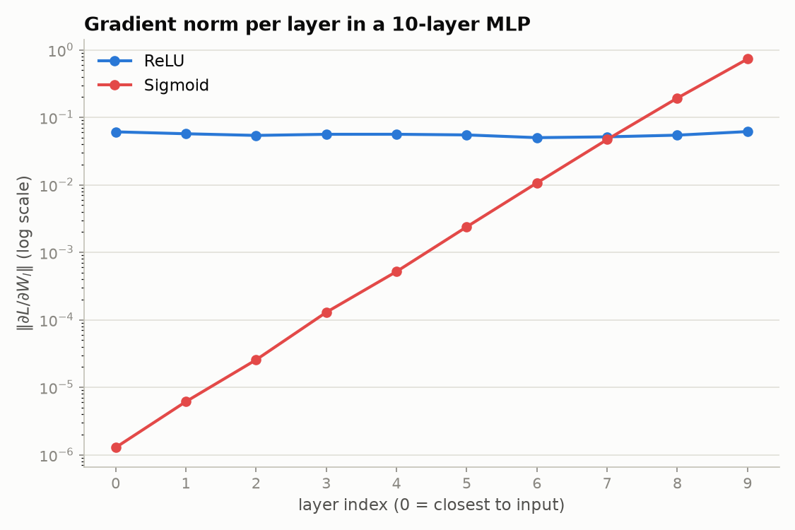
With sigmoid, the gradient norm at layer 9 (closest to the output) is \(0.73\) , while at layer 0 (closest to the input) it is only \(1.3\times 10^{-6}\) — a decay of roughly 570,000× (ratio \(1.7\times10^{-6}\) ). This is exactly the effect predicted by equation (17): a factor of \(\sigma'\le 0.25\) multiplying in at every one of the 10 layers. With ReLU, layer 0 is \(0.061\) and layer 9 is \(0.062\) — essentially the same magnitude (ratio \(0.99\) ) — confirming that a constant derivative of \(1\) in the positive region prevents the vanishing-gradient effect.
This is why deep networks overwhelmingly use ReLU (or its variants) rather than sigmoid for hidden-layer activations: when gradients vanish near the input, those layers’ parameters barely update, and training effectively stalls. Vanishing gradients are also mitigated by mechanisms beyond activation-function choice, such as LSTM gating , residual connections, and adaptive optimizers like Adam .
Experiment
With the theory established, we train the Model class defined above (ReLU hidden activations) on a simple regression task, \(f(x) = x^2 + 2x + 1\)
.
# Create test data
def math(x):
    return x*x + 2*x + 1

def make():
    x = np.random.rand(1000)
    y = math(x)
    return x,y

train_x, train_y = make()
test_x, test_y = make()
model = Model(1,1)

# Evaluate on test data before training
gosa = 0
for i in range(1000):
    output = model(torch.tensor([[float(test_x[i])]]))
    gosa += abs((output - test_y[i]))

print("Mean error before training:", gosa/1000)

# Train on training data
for i in range(1000):
    output = model(torch.tensor([[float(train_x[i])]]))
    loss = model.update(output, torch.tensor([[float(train_y[i])]]))

# Evaluate on test data after training
gosa = 0
for i in range(1000):
    output = model(torch.tensor([[float(test_x[i])]]))
    gosa += abs((output - test_y[i])[0])

print("Mean error after training:", gosa/1000)
Output (with torch.manual_seed(0) and np.random.seed(0) fixed):
Mean error before training: tensor([[2.4819]], grad_fn=<DivBackward0>)
Mean error after training: tensor([0.0326], grad_fn=<DivBackward0>)
After just 1000 steps of SGD, the mean absolute error on the test set drops from \(2.48\) to \(0.033\) — roughly a 75-fold reduction. Behind this improvement is exactly the chain-rule gradient computation derived in equations (5)–(12) of this article.
Related Articles
- Training Neural Networks with Genetic Algorithms in Python - Optimizing NN weights using evolutionary methods instead of gradient descent
- From SGD to Adam: Evolution of Gradient-Based Optimization - Optimizers (SGD, Momentum, Adam, …) that consume the gradients derived in this article
- Understanding Self-Attention from Scratch: Math and Python Implementation - The core mechanism of Transformers. Unlike this article’s elementwise activations, softmax is not applied elementwise, so its Jacobian is non-diagonal — a useful contrast
- LSTM for Time Series Forecasting: Theory and Python Implementation - How LSTM’s gating mechanism mitigates vanishing gradients
References
- Rumelhart, D. E., Hinton, G. E., & Williams, R. J. (1986). “Learning representations by back-propagating errors.” Nature, 323(6088), 533-536.
- Goodfellow, I., Bengio, Y., & Courville, A. (2016). Deep Learning. MIT Press. Chapter 6.
- Glorot, X., & Bengio, Y. (2010). “Understanding the difficulty of training deep feedforward neural networks.” AISTATS 2010.
- PyTorch Documentation:
torch.autograd. https://pytorch.org/docs/stable/autograd.html