1. What Is Bayes’ Theorem
In one sentence, Bayes’ theorem is the rule for how to update a belief (a probability estimate) after seeing new evidence (data). How to interpret a health screening result, how to flag a spam email, how to judge whether a coin is biased — different as these problems look, they all reduce to the same single equation.
For events \(A\) and \(B\) , Bayes’ theorem is written as follows.
\[ P(A \mid B) = \frac{P(B \mid A)\, P(A)}{P(B)} \tag{1} \]Each of the four terms in equation (1) has a name.
- \(P(A)\) : the prior probability (prior distribution) — how plausible \(A\) seemed before seeing data \(B\) .
- \(P(B \mid A)\) : the likelihood — how likely we would be to observe data \(B\) , assuming \(A\) is true.
- \(P(B)\) : the marginal likelihood (evidence) — how likely data \(B\) is overall, regardless of whether \(A\) is true. It acts as a normalizing constant.
- \(P(A \mid B)\) : the posterior probability (posterior distribution) — our updated belief about \(A\) after seeing data \(B\) .
In other words, Bayes’ theorem takes the prior probability, reweights it by how strongly the data supports it (the likelihood), and normalizes by how likely the data was in the first place (the marginal likelihood), producing the posterior probability. The rest of this article walks through two worked examples — a diagnostic test and a sequence of coin flips — to see exactly how these four terms interact in practice.
2. Deriving It From Conditional Probability
Bayes’ theorem is not a separate axiom; it follows in two lines from the definition of conditional probability. The two definitions are:
\[ P(A \mid B) = \frac{P(A \cap B)}{P(B)}, \qquad P(B \mid A) = \frac{P(A \cap B)}{P(A)} \tag{2} \]Solving the right-hand equation for \(P(A \cap B)\) gives \(P(A \cap B) = P(B \mid A)\,P(A)\) . Substituting this into the numerator of the left-hand equation yields
\[ P(A \mid B) = \frac{P(B \mid A)\,P(A)}{P(B)} \]which is exactly equation (1). All we did was write the “joint probability” \(P(A \cap B)\) two different ways — once conditioning on \(A\) , once on \(B\) — and set them equal. No extra assumption is needed anywhere in this derivation, and that simplicity is one reason Bayes’ theorem shows up in so many places.
3. Worked Example 1: Diagnostic Testing and Positive Predictive Value
The power of Bayes’ theorem is easiest to feel in the interpretation of a medical test. Consider the following setup.
- Disease prevalence (the fraction of the tested population that actually has the disease): 1%
- Sensitivity (the probability a sick person tests positive): 90%
- Specificity (the probability a healthy person tests negative): 95%
Given this, what is the probability that someone who tests positive actually has the disease (the positive predictive value, PPV)? The intuitive guess is “90% sensitivity, so about 90% likely” — but the actual calculation gives a very different answer.
Let \(D\) denote “has the disease” and \(T^+\) denote “tests positive.” Applying Bayes’ theorem:
\[ P(D \mid T^+) = \frac{P(T^+ \mid D)\,P(D)}{P(T^+)} \]The marginal likelihood \(P(T^+)\) in the denominator is found by summing over the diseased and non-diseased cases:
\[ P(T^+) = P(T^+ \mid D)\,P(D) + P(T^+ \mid \bar{D})\,P(\bar{D}) \]Substituting the numbers — \(P(D) = 0.01\) , \(P(T^+ \mid D) = 0.90\) (sensitivity), \(P(T^+ \mid \bar{D}) = 1 - 0.95 = 0.05\) (one minus specificity), \(P(\bar{D}) = 0.99\) — gives
\[ P(T^+) = 0.90 \times 0.01 + 0.05 \times 0.99 = 0.009 + 0.0495 = 0.0585 \] \[ P(D \mid T^+) = \frac{0.009}{0.0585} = 0.1538\ldots \approx \mathbf{15.4\%} \]Despite a 90%-sensitive test coming back positive, the probability of actually having the disease is only 15.4%. This is not because the test is bad — it’s because the prevalence is only 1%. Out of the huge healthy population (99%), just a 5% false-positive rate is enough to produce more false positives than the small number of true positives. Judging by the likelihood (sensitivity) alone, while ignoring the prior (prevalence), leads straight into this trap.
The same calculation, applied to a population of 100,000, gives the following contingency table.
| Test Positive | Test Negative | Total | |
|---|---|---|---|
| Has disease | 900 | 100 | 1,000 |
| No disease | 4,950 | 94,050 | 99,000 |
| Total | 5,850 | 94,150 | 100,000 |
Of the 1,000 people who have the disease, 90% sensitivity gives 900 true positives (TP) and 100 false negatives (FN). Of the 99,000 healthy people, the 5% false-positive rate (1 − specificity) gives 4,950 false positives (FP) and 94,050 true negatives (TN). The positive predictive value is
\[ \mathrm{PPV} = \frac{\mathrm{TP}}{\mathrm{TP} + \mathrm{FP}} = \frac{900}{900 + 4{,}950} = \frac{900}{5{,}850} = 0.1538\ldots \approx 15.4\% \]which matches the earlier calculation. Incidentally, the negative predictive value (NPV, the probability that someone who tests negative is actually healthy) works out to \(94{,}050 / 94{,}150 \approx 99.9\%\) — very high. This test is one where “a positive result should not be taken at face value, but a negative result can be trusted.” When reading screening test results in a low-prevalence population, keeping this asymmetry between PPV and NPV in mind is essential.
4. Worked Example 2: The Sequential Nature of Bayesian Updating
Another key aspect of Bayes’ theorem is that each time new data arrives, the current posterior can be used as the prior for the next update — beliefs can be revised sequentially. We illustrate this with a biased coin, estimating the probability \(\theta\) that it lands heads.
As a prior for \(\theta\) , we use Beta(1,1), which is equivalent to a uniform distribution on \([0,1]\) . The Beta distribution has probability density function
\[ p(\theta \mid \alpha, \beta) \propto \theta^{\alpha - 1}(1-\theta)^{\beta - 1} \]Flipping the coin once, the likelihood of heads is \(P(\text{Head} \mid \theta) = \theta\) , and the likelihood of tails is \(P(\text{Tail} \mid \theta) = 1-\theta\) . Starting from a prior \(\mathrm{Beta}(\alpha, \beta)\) , observing a head gives the posterior
\[ p(\theta \mid \text{Head}) \propto \theta \cdot \theta^{\alpha-1}(1-\theta)^{\beta-1} = \theta^{\alpha}(1-\theta)^{\beta-1} \;\Rightarrow\; \mathrm{Beta}(\alpha+1,\ \beta) \]so the posterior is again a Beta distribution, just with one exponent incremented. A tail increments \(\beta\) in the same way. In general, after \(n\) trials with \(k\) heads and \(n-k\) tails,
\[ \mathrm{Beta}(\alpha, \beta) \xrightarrow{\ k\text{ heads}, (n-k)\text{ tails}\ } \mathrm{Beta}(\alpha + k,\ \beta + n - k) \tag{3} \]To make this concrete, we simulated a single coin (fixed random seed, true head probability \(p=0.65\) ), starting from Beta(1,1) and updating one flip at a time. The table below shows the first ten updates.
| Trial \(n\) | Outcome | Posterior | Posterior mean \(\alpha/(\alpha+\beta)\) |
|---|---|---|---|
| 0 | – | Beta(1,1) | 0.500 |
| 1 | Head | Beta(2,1) | 0.667 |
| 2 | Tail | Beta(2,2) | 0.500 |
| 3 | Head | Beta(3,2) | 0.600 |
| 4 | Tail | Beta(3,3) | 0.500 |
| 5 | Head | Beta(4,3) | 0.571 |
| 6 | Head | Beta(5,3) | 0.625 |
| 7 | Tail | Beta(5,4) | 0.556 |
| 8 | Head | Beta(6,4) | 0.600 |
| 9 | Head | Beta(7,4) | 0.636 |
| 10 | Head | Beta(8,4) | 0.667 |
The posterior moves with every single flip. What matters is that repeating this “use the posterior as the next prior” procedure any number of times gives exactly the same final posterior as plugging all the data into equation (3) at once. This is because the likelihood factors as a product over trials, \(\theta^{k}(1-\theta)^{n-k}\) , which does not depend on the order of multiplication — so processing observations one at a time (online learning) and processing them all together (batch processing) are guaranteed to reach the same conclusion.
Continuing to flip the same coin and comparing the posterior at \(n = 10, 50, 200\) gives the following (the head/tail counts are all from the same simulation).
| Trials \(n\) | Heads/Tails | Posterior | Posterior mean | Posterior std. dev. |
|---|---|---|---|---|
| 0 (prior) | – | Beta(1,1) | 0.500 | 0.289 |
| 10 | 7 heads / 3 tails | Beta(8,4) | 0.667 | 0.131 |
| 50 | 34 heads / 16 tails | Beta(35,17) | 0.673 | 0.064 |
| 200 | 130 heads / 70 tails | Beta(131,71) | 0.649 | 0.034 |
As data accumulates, the posterior mean converges toward the true value \(p=0.65\) , and the posterior standard deviation (the spread of the distribution, i.e. the uncertainty) shrinks monotonically. This is visualized below.
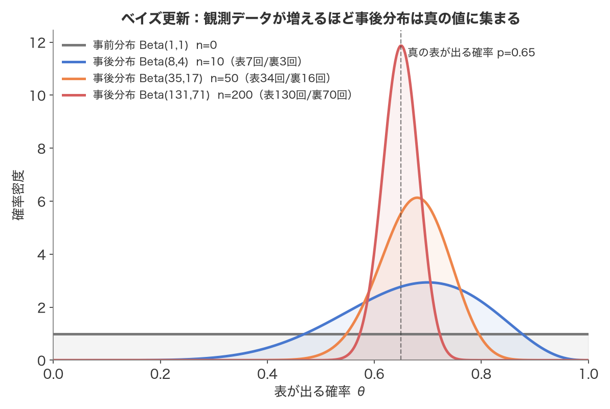
The prior’s gentle, wide hump (high variance, meaning we know very little) turns into an increasingly sharp peak as more data is folded in. This is the essence of Bayesian updating, and a concrete instance of the relationship “posterior ∝ likelihood × prior” discussed next.
5. How Prior, Posterior, and Likelihood Relate
Because the denominator \(P(B)\) in equation (1) is a constant that does not depend on \(A\) (a normalizing constant), focusing on proportionality alone lets us write
\[ \text{posterior} \;\propto\; \text{likelihood} \times \text{prior} \]In the coin-flip example above, this relation showed up directly as \(p(\theta \mid \text{data}) \propto p(\text{data} \mid \theta)\, p(\theta)\) . When the prior is a Beta distribution and the likelihood is Bernoulli/binomial, the posterior is again a Beta distribution — and whenever a prior and the resulting posterior belong to the same family of distributions for a given likelihood, that prior is called a conjugate prior. Some well-known conjugate pairs are:
- Beta × binomial (Bernoulli) likelihood → posterior is also Beta (the coin-flip example in this article)
- Gamma × Poisson likelihood → posterior is also Gamma (e.g. estimating an event rate per unit time)
- Normal × Normal likelihood (known variance) → posterior is also Normal (e.g. estimating a mean)
The biggest benefit of choosing a conjugate prior is that the shape and parameters of the posterior can be derived analytically (in closed form), without any numerical integration. Well-known conjugate pairs already exist for the distributions used most often in practice, so it’s worth checking whether one applies before reaching for anything heavier. That said, once a model grows complex enough that the likelihood and prior are no longer conjugate, the posterior can no longer be found analytically — how to handle that situation is covered in Section 7.
6. Bayesian vs. Frequentist Statistics
Frequentist statistics is often contrasted with Bayesian statistics. In practice, it’s more useful to think of the two not as opposing camps, but as differing in how they interpret the concept of probability, and in the resulting toolkit.
In frequentist statistics, probability is defined as “the limit of the relative frequency of an event over infinitely many repeated trials under identical conditions.” A population parameter (say, a coin’s true probability of heads) is unknown but treated as a fixed constant; the data, not the parameter, is what has a probability distribution. Estimation relies on tools like point estimates, confidence intervals, and hypothesis testing (p-values).
In Bayesian statistics, probability is defined as “a degree of belief in a proposition.” The parameter itself is treated as uncertain, that uncertainty is expressed explicitly as a prior distribution, and it is updated into a posterior distribution each time new data arrives. The result of inference is not a single point estimate but an entire distribution, from which a credible interval can be derived. A credible interval can be interpreted directly as “there is a 95% probability the parameter lies in this interval,” whereas a frequentist confidence interval carries a subtly different interpretation — “if this procedure were repeated many times, 95% of the resulting intervals would contain the true value.” This distinction is worth keeping in mind.
Which one to use depends on the goal. For large, standardized A/B tests, or clinical trials that must be submitted to a regulator, frequentist hypothesis testing — with its established procedures and easy reproducibility checks — is widely used. On the other hand, when data is scarce and prior knowledge should be leveraged actively, when decisions need to be updated sequentially, or when the estimate itself needs to feed downstream decisions as a full probability distribution, the Bayesian approach plays to its strengths. This is not a question of which is superior, but of choosing the right tool for the situation.
7. Connections to Machine Learning and Practice
Bayes’ theorem is not just theory — it’s used widely in practice.
The most familiar application is the naive Bayes classifier. Take spam filtering as an example: given the words \(x_1, \dots, x_d\) in an email, the posterior probability of a class \(y\) (spam or legitimate) can be written
\[ P(y \mid x_1,\dots,x_d) \propto P(y) \prod_{i=1}^{d} P(x_i \mid y) \]Words in an email are, of course, correlated with each other, but the simplifying (naive) assumption that “words are conditionally independent given the class” makes this probability fast to compute even from a small training set. Because of this simplicity, naive Bayes remains a widely used baseline for text classification today.
Many real-world models, though, do not have the conjugacy discussed in Section 5, so their posterior cannot be written down analytically. High-dimensional Bayesian linear models with hundreds of regression coefficients, and hierarchical models, are typical examples. In such cases, Markov chain Monte Carlo (MCMC) methods are used to approximate the posterior’s shape by drawing samples directly from it. The basic Metropolis algorithm loses efficiency on high-dimensional distributions with strong correlation between variables — a weakness overcome using gradient information by Hamiltonian Monte Carlo (HMC), covered in https://yuhi-sa.github.io/en/posts/20260715_hamiltonian_monte_carlo/1/. A single equation — Bayes’ theorem — runs all the way from a simple probability calculation to a modern Bayesian inference engine.
Recommended Reading
For readers who want to build a systematic understanding of Bayesian thinking within a machine learning framework, the following book is a good starting point.
A broader list of standard Python and machine learning references is collected in 12 Recommended Books for Learning Signal Processing, Machine Learning, and Control in Python (2026, by Level) .
Summary
Bayes’ theorem, \(P(A \mid B) = P(B \mid A)P(A) / P(B)\) , follows in two lines from the definition of conditional probability, yet it offers a general-purpose way of “updating beliefs based on evidence” through its three components — prior, likelihood, and posterior. The diagnostic test example showed how ignoring the prior probability (the prevalence) can lead to a counterintuitive result being overlooked. The coin-flip example used the conjugacy of the Beta distribution to trace, with real numbers, how the posterior converges toward the true value as data accumulates and uncertainty shrinks. From naive Bayes to MCMC, a wide swath of machine learning rests on this single equation.
FAQ
Q. What is Bayes’ theorem used for? A. It’s used anywhere a probability estimate needs to be updated in light of new data: spam filtering (naive Bayes), interpreting health screening and diagnostic test results, sequential decision-making in A/B testing, anomaly detection, and training machine learning models via Bayesian inference.
Q. How do you choose a prior distribution? A. If past data or expert knowledge is available, use it to construct an informative prior (in this article’s example, “1% prevalence” plays that role). When there is no strong prior knowledge, an uninformative prior such as a uniform distribution is often used instead. Choosing a conjugate prior (Section 5) also has the practical benefit of making the computation tractable. In every case, as more data accumulates the likelihood comes to dominate, and the choice of prior matters less and less (as shown in the figure in Section 4).
Q. Should I use Bayesian or frequentist methods? A. Neither is simply “better” — the right choice depends on the goal. Frequentist hypothesis testing is widely used for standardized, large-scale testing and situations where reproducibility needs to be verified, while the Bayesian approach plays to its strengths when data is scarce and prior knowledge should be leveraged, or when decisions need to be updated sequentially (Section 6).
Related Articles
- Fundamentals of Probability - Joint, marginal, and conditional probability — the probability-theory foundations this article builds on
- Bayesian Linear Regression: From Least Squares to Bayesian Estimation - Applying Bayes’ theorem to parameter estimation in a regression model
- MCMC Fundamentals: Metropolis Algorithm and Gibbs Sampling - Sampling methods for approximating posteriors that lack conjugacy
- Hamiltonian Monte Carlo (HMC) in Python - An advanced technique that uses gradient information to make MCMC more efficient
- Moments in Statistics: Indicators that Characterize Probability Distributions - The statistical measures, like mean and variance, used to summarize a posterior distribution