To understand why the EM algorithm is able to increase the log-likelihood, we introduce the concepts of the “Evidence Lower Bound (ELBO)” and “KL Divergence (Kullback-Leibler Divergence).”
Evidence Lower Bound (ELBO)
The Evidence Lower Bound \(\mathcal{L}(\theta, \hat{\theta})\) in the EM algorithm is defined as:
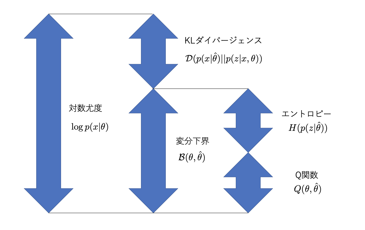
\[ \mathcal{L}(\theta, \hat{\theta}) = \int p(z|x,\hat{\theta}) \log \frac{p(x,z|\theta)}{p(z|x,\hat{\theta})}dz \]This expression is derived from the relationship between the log-likelihood \(\log p(x|\theta)\) and the KL divergence between the posterior distributions \(p(z|x,\hat{\theta})\) and \(p(z|x,\theta)\) of the latent variable \(z\).
\[ \log p(x|\theta) = \mathcal{L}(\theta, \hat{\theta}) + KL(p(z|x,\hat{\theta}) || p(z|x,\theta)) \]Here:
- \(\mathcal{L}(\theta, \hat{\theta})\) is the Evidence Lower Bound (ELBO).
- \(KL(p(z|x,\hat{\theta}) || p(z|x,\theta))\) is the KL divergence.
The ELBO \(\mathcal{L}(\theta, \hat{\theta})\) can also be expressed as the sum of the Q function computed in the E-step and the entropy of the posterior distribution of the latent variables.
\[ \mathcal{L}(\theta, \hat{\theta}) = Q(\theta, \hat{\theta}) + H(p(z|x,\hat{\theta})) \]KL Divergence
KL divergence \(KL(q||p)\) is a measure of the “information-theoretic distance” between two probability distributions \(q(x)\) and \(p(x)\).
\[ KL(q||p) = \mathbb{E}\_q[\log\frac{q(x)}{p(x)}] = \int q(x)\log \frac{q(x)}{p(x)}dx \]KL divergence has the following properties:
- It is always non-negative: \(KL(q||p) \ge 0\)
- It equals zero only when the two distributions are identical: \(KL(q||p) = 0 \iff q(x) = p(x)\)
The EM Algorithm and Monotonic Increase of the ELBO
Each step of the EM algorithm monotonically increases the log-likelihood. This can be explained through the relationship between the ELBO and KL divergence.
E-step: Fix the current parameters \(\hat{\theta}\) and compute the posterior distribution \(p(z|x,\hat{\theta})\) of the latent variables \(z\). In this step, \(\theta\) is updated so that the KL divergence is minimized (becomes 0), meaning \(p(z|x,\hat{\theta})\) matches \(p(z|x,\theta)\). This causes the ELBO \(\mathcal{L}(\theta, \hat{\theta})\) to equal the log-likelihood \(\log p(x|\theta)\).
M-step: Using \(p(z|x,\hat{\theta})\) computed in the E-step, find the new parameter \(\theta\) that maximizes the Q function \(Q(\theta, \hat{\theta})\). Maximizing the Q function also increases the ELBO \(\mathcal{L}(\theta, \hat{\theta})\). Since the KL divergence is non-negative, the log-likelihood \(\log p(x|\theta)\) also increases.
In this way, the EM algorithm monotonically increases the log-likelihood by alternating between the E-step and M-step.
References
- Taro Tezuka, Understanding Bayesian Statistics and Machine Learning, Kodansha (2017)