Variational Autoencoder (VAE)

The Variational Autoencoder (VAE) is a type of generative model that aims to learn the latent structure of data and generate new data. Similar to how the EM algorithm maximizes the log-likelihood lower bound (see The EM Algorithm ), VAE also learns by maximizing the Evidence Lower Bound (ELBO).

A key feature of VAE is that it has a probabilistic encoder (recognition model) and a probabilistic decoder (generative model). This makes the latent space smooth and enables meaningful data generation.

• Recognition model (encoder): Estimates the probability distribution \(q_\phi(z|x)\) of latent variables \(z\) from input data \(x\) . It has parameters \(\phi\) .
• Generative model (decoder): Generates the probability distribution \(p_\theta(x|z)\) of data \(x\) from latent variables \(z\) . It has parameters \(\theta\) .

The latent variable \(z\) can be interpreted as a lower-dimensional, abstract “latent representation” or “latent code” of the information contained in input data \(x\) .

Autoencoder

An autoencoder is a neural network that learns to compress and encode input data, then reconstruct (decode) it to output the same content as the input. The intermediate layer (latent space) becomes a compressed representation (code) that captures the important features of the input data.

VAE introduces the concept of variational inference into this autoencoder framework.

Deriving the ELBO for VAE

VAE’s goal is to maximize the marginal likelihood \(p_\theta(x) = \int p_\theta(x|z)p(z)dz\) , but the integral over the latent variable \(z\) is generally intractable. We apply the same Jensen’s-inequality argument used in the EM algorithm article ( The EM Algorithm ), this time using the recognition model \(q_\phi(z|x)\) .

(This is Jensen’s inequality, applied because the logarithm is concave.) As with EM, the gap between the log-likelihood and the ELBO can be evaluated exactly as a KL divergence.

Since \(KL \ge 0\) , \(\mathcal{L}(\theta,\phi;x)\) is a lower bound on the log-likelihood (the ELBO), and equality holds only when \(q_\phi(z|x)=p_\theta(z|x)\) (i.e., matches the true posterior exactly). The difference from EM is that EM computes the exact posterior \(p(z|x,\hat\theta)\) separately for each data point, whereas VAE approximates \(q_\phi(z|x)\) with a neural network and performs inference for all data points jointly, sharing a single set of parameters \(\phi\) (amortized inference). This removes the need for exact posterior computation, but at the cost of a persistent gap (\(KL>0\) ) between \(q_\phi\) and the true posterior.

Expanding the ELBO gives the familiar two-term decomposition.

(obtained by substituting \(p_\theta(x,z) = p_\theta(x|z)p(z)\) and rearranging \(\mathbb{E}_{q_\phi(z|x)}[\log p_\theta(x,z)] - \mathbb{E}_{q_\phi(z|x)}[\log q_\phi(z|x)]\) .)

1. Reconstruction error (first term): \(\mathbb{E}_{q_\phi(z|x)}[\log p_\theta(x|z)]\) This represents how accurately the decoder can reconstruct the original input \(x\) using the latent variable \(z\) generated by the encoder. Maximizing this term corresponds to minimizing the reconstruction error.

2. Regularization term (second term): \(KL(q_\phi(z|x) \| p(z))\) This measures how close the distribution \(q_\phi(z|x)\) of latent variables \(z\) estimated by the encoder is to the predefined prior distribution \(p(z)\) of the latent variables. Minimizing this term serves to make the latent space smooth and enable meaningful data generation.

Recognition Model \(q_\phi(z|x)\)

The recognition model estimates the distribution of latent variables \(z\) from input \(x\) . Typically, a neural network is used to output the mean \(\mu(x)\) and variance \(\sigma^2(x)\) (or log-variance \(\log \sigma^2(x)\) ) of the multivariate normal distribution that \(z\) follows.

Here, \(\mu_\phi(x)\) and \(\sigma^2_\phi(x)\) are outputs of the neural network that takes input \(x\) .

Generative Model \(p_\theta(x|z)\) and the Reconstruction Term for a Gaussian Decoder

The generative model produces the distribution of data \(x\) from latent variables \(z\) . The choice of probability distribution depends on the type of data \(x\) .

• Binary data (e.g., black-and-white images): Bernoulli distribution (or categorical distribution)
• Continuous data (e.g., grayscale images): Gaussian distribution

For continuous data, a multivariate normal distribution with fixed variance is commonly used:

Here, \(\nu_\theta(z)\) is the output of the neural network that takes latent variable \(z\) as input. Computing the reconstruction term explicitly in this case shows it is equivalent to a mean-squared-error (MSE) loss. For \(D\) -dimensional data \(x\) ,

The first term on the right-hand side does not depend on \(z\) and can be dropped when maximizing the ELBO over \(\theta,\phi\) , giving

In other words, maximizing the reconstruction term is the same, up to a constant scaling and a sign, as minimizing the mean squared error between the decoder output \(\nu_\theta(z)\) and the input \(x\) . In practice, “using MSE as the reconstruction loss” implicitly assumes a Gaussian decoder with fixed variance.

Prior Distribution of Latent Variables \(p(z)\) and the Closed-Form KL Divergence

The prior distribution of latent variables is typically defined as a product of standard normal distributions (mean 0, variance 1).

This prior is fixed during training and does not depend on parameters \(\theta\) or \(\phi\) . Because both \(q_\phi(z|x)\) and \(p(z)\) are Gaussian, the KL divergence regularization term can be computed in closed form, without any integral. We derive the 1-dimensional case (\(q=\mathcal{N}(\mu,\sigma^2)\) , \(p=\mathcal{N}(0,1)\) ) explicitly.

Since \(\log q(z) = -\frac{1}{2}\log(2\pi\sigma^2) - \frac{(z-\mu)^2}{2\sigma^2}\) and \(\mathbb{E}_q[(z-\mu)^2]=\sigma^2\) ,

Similarly, since \(\log p(z) = -\frac{1}{2}\log(2\pi) - \frac{z^2}{2}\) and \(\mathbb{E}_q[z^2] = \sigma^2+\mu^2\) (from the definition of variance, \(\text{Var}(z)=\mathbb{E}[z^2]-\mu^2\) ),

Taking the difference:

Since each dimension of \(q_\phi(z|x)\) is independent (diagonal covariance), the multivariate case is just the sum of this term over dimensions.

The fact that this expression can be written in closed form, with no integral required, is one of the main reasons VAE training is practical (the reconstruction term must be approximated via Monte Carlo sampling, but the KL term can be computed exactly).

Gradient Descent and the Reparameterization Trick

VAE training uses gradient descent (optimization algorithms such as Adam) to update parameters \(\theta\) and \(\phi\) to maximize the ELBO \(\mathcal{L}(\theta, \phi)\) .

The gradient of the reconstruction term is relatively straightforward to compute, but the expectation \(\mathbb{E}_{q_\phi(z|x)}[\cdot]\) is itself taken over a distribution that depends on \(\phi\) . If we naively sample \(z\sim q_\phi(z|x)\) via Monte Carlo and try to differentiate through it, the sampling operation blocks gradient flow back to \(\phi\) .

To solve this problem, the reparameterization trick is used. This technique represents the latent variable \(z\) using a random variable \(\epsilon\) that does not depend on parameter \(\phi\) and a deterministic function \(g(\epsilon, x, \phi)\) that depends on \(\phi\) . For a Gaussian, \(z = \mu_\phi(x) + \sigma_\phi(x) \cdot \epsilon\) (where \(\epsilon \sim \mathcal{N}(0, I)\) ). The full mathematical details of the trick, and its generalization to multivariate and non-Gaussian distributions, are covered in The Reparameterization Trick — see that article for a deeper dive.

Here, we add a point not covered there: the trick is not merely about making sampling differentiable — it also has the practically decisive benefit of substantially reducing the variance of the gradient estimate. The natural point of comparison is another general technique for differentiating through an expectation over a sampling operation, the score-function estimator (REINFORCE):

This estimator is general enough to work even when \(f\) is not differentiable, but because the value of \(f(z)\) itself multiplies the gradient weight, its variance tends to be large whenever \(f(z)\) has high variance. The reparameterization-trick gradient, in contrast,

directly uses the gradient information of \(f\) (a pathwise derivative), and is known both empirically and theoretically to have lower variance whenever \(f\) is smooth (Kingma & Welling, 2014; Rezende et al., 2014). Since VAE decoders are typically differentiable neural networks, this is exactly the setting where the low-variance reparameterization gradient applies.

Executed Python Verification: Training a Linear-Gaussian VAE with Hand-Derived Gradients

To verify ELBO maximization hands-on, we implement everything without a neural-network library such as PyTorch — every gradient is derived by hand from the formulas above and implemented in pure NumPy. We simplify the encoder and decoder to linear maps (“linear-Gaussian VAE”) and train on 2-dimensional data generated from a 1-dimensional latent variable.

Data-generating process: from a true latent variable \(z^* \sim \mathcal{N}(0,1)\) , we generate 2D data \(x = z^* w^* + (1,-0.5) + \text{noise}\) (with \(\text{noise}\sim\mathcal{N}(0,0.3^2 I)\) ) using a true direction vector \(w^*=(2,1)\) and offset \((1,-0.5)\) .

Model: \(\mu_\phi(x)=w_\mu^\top x + b_\mu\) , \(\log\sigma^2_\phi(x) = w_{lv}^\top x + b_{lv}\) (both scalar outputs), \(\nu_\theta(z) = w_{dec}\,z + b_{dec}\) (2D output), with the decoder variance fixed at \(\sigma_x^2=0.3^2\) .

Deriving the gradients: the loss \(L=-\mathcal{L}\) (the negative ELBO, per sample), using the reparameterization \(z=\mu+\sigma\epsilon\) (with \(\sigma=\exp(\frac12\log\sigma^2)\) ), is

Working backward through the chain rule gives the following gradients (writing \(d(\cdot)\) for the gradient of \(L\) ):

(the second terms \(\mu\) in \(d\mu\) , and \(\tfrac12(e^{\log\sigma^2}-1)\) in \(d\log\sigma^2\) , are the contributions from differentiating the KL term with respect to \(\mu\) and \(\log\sigma^2\) , respectively.)

import numpy as np

rng = np.random.default_rng(0)

N = 500
true_direction = np.array([2.0, 1.0])
z_true = rng.normal(0, 1, size=N)
noise = rng.normal(0, 0.3, size=(N, 2))
X = z_true[:, None] * true_direction[None, :] + noise + np.array([1.0, -0.5])

sigma_x2 = 0.3**2

w_mu = rng.normal(0, 0.1, size=2); b_mu = 0.0
w_lv = rng.normal(0, 0.1, size=2); b_lv = 0.0
w_dec = rng.normal(0, 0.1, size=2); b_dec = rng.normal(0, 0.1, size=2)

lr = 0.005
n_epochs = 400
elbo_history = []

for epoch in range(n_epochs):
    eps = rng.normal(size=N)
    mu = X @ w_mu + b_mu
    logvar = np.clip(X @ w_lv + b_lv, -8, 8)
    sigma = np.exp(0.5 * logvar)
    z = mu + sigma * eps

    xhat = z[:, None] * w_dec[None, :] + b_dec
    recon = (1.0 / (2 * sigma_x2)) * np.sum((X - xhat) ** 2, axis=1)
    kl = 0.5 * (np.exp(logvar) + mu**2 - 1 - logvar)
    elbo_history.append(-(recon + kl).mean())

    d_xhat = -(1.0 / sigma_x2) * (X - xhat)
    d_w_dec = (d_xhat * z[:, None]).mean(axis=0)
    d_b_dec = d_xhat.mean(axis=0)
    d_z = d_xhat @ w_dec

    d_mu = d_z + mu
    d_logvar = d_z * eps * 0.5 * sigma + 0.5 * (np.exp(logvar) - 1)

    d_w_mu = (d_mu[:, None] * X).mean(axis=0)
    d_b_mu = d_mu.mean()
    d_w_lv = (d_logvar[:, None] * X).mean(axis=0)
    d_b_lv = d_logvar.mean()

    w_dec -= lr * d_w_dec; b_dec -= lr * d_b_dec
    w_mu  -= lr * d_w_mu;  b_mu  -= lr * d_b_mu
    w_lv  -= lr * d_w_lv;  b_lv  -= lr * d_b_lv

print(f"epoch   1: ELBO = {elbo_history[0]:.4f}")
print(f"epoch  10: ELBO = {elbo_history[9]:.4f}")
print(f"epoch  50: ELBO = {elbo_history[49]:.4f}")
print(f"epoch 100: ELBO = {elbo_history[99]:.4f}")
print(f"epoch 400: ELBO = {elbo_history[-1]:.4f}")

The executed output is:

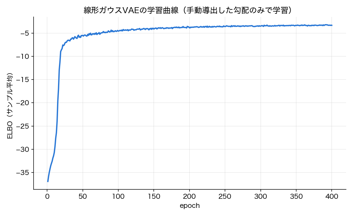
epoch   1: ELBO = -36.9169
epoch  10: ELBO = -30.7112
epoch  50: ELBO = -5.4867
epoch 100: ELBO = -4.5815
epoch 400: ELBO = -3.3315

Using only hand-derived gradients, the ELBO improves in a near-monotonic fashion from \(-36.92\) to \(-3.33\) . Comparing the trained parameters against the true data-generating process:

true decoder direction   w* = [2.0, 1.0]
learned decoder weight w_dec = [-1.4122, -0.7163]
cosine similarity(w_dec, w*) = -1.0000
learned b_dec = [0.804, -0.6096]  (true offset = [1.0, -0.5])
corr(encoder mean mu(x), true latent z_true) = -0.9920

The correlation between the encoder output \(\mu(x)\) and the true latent variable \(z^*\) is a very strong \(-0.992\) , confirming that the latent variable has been correctly recovered. Notice, though, that the cosine similarity is exactly \(-1.0\) — the learned direction vector is precisely the negative of the true direction. This is not a bug; it is the sign non-identifiability of latent-variable models discussed in the edge case below.

Visualizing the training curve:

Edge Cases and Caveats

• Non-identifiability of the latent variable (sign and rotation ambiguity): as our experiment above confirmed, simultaneously flipping \(z \to -z\) and \(w_{dec} \to -w_{dec}\) leaves the likelihood \(p_\theta(x|z)\) unchanged (more generally, the model is invariant under any linear transformation \(z \to Az\) , \(w_{dec} \to w_{dec}A^{-1}\) ). This is normally a harmless form of non-identifiability, but Wang, Blei & Cunningham (2023) show theoretically that when this non-identifiability becomes extreme, it can lead to posterior collapse — where the encoder ignores the input \(x\) entirely, collapsing to \(q_\phi(z|x) \approx p(z)\) , so the latent representation loses all meaning. This is known to occur especially often when the decoder is highly expressive (e.g., an RNN or Transformer that can reconstruct a sequence via autoregression alone, without needing \(z\) at all).
• KL vanishing and its mitigations: when posterior collapse occurs, the regularization term \(KL(q_\phi(z|x)\|p(z))\) approaches zero and \(z\) stops carrying any information about the input. Common mitigations include KL annealing (starting with a small weight on the KL term early in training and gradually increasing it) and free bits (imposing a floor on the KL term).
• Choice of decoder variance \(\sigma_x^2\) : as shown in the derivation above, fixing \(\sigma_x^2\) reduces the reconstruction term to an MSE loss, but increasing \(\sigma_x^2\) shrinks the relative weight of the reconstruction term, making the KL (regularization) term more dominant. In effect, \(\sigma_x^2\) acts as a hyperparameter controlling the balance against the KL term — playing a role similar to the \(\beta\) in \(\beta\) -VAE.

References

• Taro Tezuka, Understanding Bayesian Statistics and Machine Learning , Kodansha (2017)
• Kingma, D. P., & Welling, M. (2014). Auto-Encoding Variational Bayes . ICLR 2014.
• Rezende, D. J., Mohamed, S., & Wierstra, D. (2014). Stochastic Backpropagation and Approximate Inference in Deep Generative Models . ICML 2014.
• Wang, Y., Blei, D. M., & Cunningham, J. P. (2023). Posterior Collapse and Latent Variable Non-identifiability . NeurIPS 2023.