In Bayesian estimation, the combination of the likelihood function and the prior distribution is crucial for obtaining the posterior distribution analytically. A prior distribution that causes the posterior distribution to have the same functional form as itself for a given likelihood function is called a conjugate prior distribution. Using conjugate priors greatly simplifies the computation of the posterior distribution.
Rather than presenting the standard conjugate pairs as a fact to memorize, this article derives the posterior distribution directly from Bayes’ theorem to show why it returns to the same functional form. We then cover the edge cases where conjugacy breaks down, and verify everything numerically in Python.
Representative Conjugate Prior Distributions
Dirichlet Distribution
The conjugate prior for the parameters (category probabilities) of the multinomial distribution is the Dirichlet distribution \(\mathcal{D}(\mu|\alpha)\) .
\[ \mathcal{D}(\mu|\alpha) = \frac{\Gamma(\sum_{j=1}^{k}\alpha_j)}{\prod_{j=1}^k\Gamma(\alpha_j)}\prod_{j=1}^k\mu_j^{\alpha_j-1} \]Here, \(\alpha = (\alpha_1, \dots, \alpha_k)\) is the parameter of the Dirichlet distribution, and \(\Gamma(\cdot)\) is the Gamma function. The Gamma function extends the concept of factorial to real numbers and is defined as:
\[ \Gamma(x) = \int_0^\infty t^{x-1}e^{-t}dt \]Beta Distribution
The conjugate prior for the parameter (success probability) of the binomial distribution is the Beta distribution \(p(\mu|a,b)\) .
\[ p(\mu|a,b) = \frac{1}{B(a,b)}\mu^{a-1}(1-\mu)^{b-1} \]Here, \(a, b\) are the parameters of the Beta distribution, and \(B(a,b)\) is the Beta function, defined as:
\[ B(a,b) = \int_0^1\mu^{a-1}(1-\mu)^{b-1}d\mu \]Gamma Distribution
The conjugate prior for the inverse of the variance (precision parameter) of the normal distribution is the Gamma distribution \(\mathcal{G}(\lambda|\kappa,\xi)\) .
\[ \mathcal{G}(\lambda|\kappa,\xi) = \frac{\xi^\kappa}{\Gamma(\kappa)}\lambda^{\kappa-1}\exp(-\xi\lambda) \]Here, \(\lambda = 1/\sigma^2\) is the precision parameter, \(\kappa\) is the shape parameter, and \(\xi\) is the scale parameter (or the inverse of the rate parameter).
Note: The conjugate prior for the mean parameter of the normal distribution is itself a normal distribution. However, if a normal distribution is used as a prior for the variance parameter, the posterior distribution does not take the form of a normal distribution, so it is not conjugate. Therefore, the precision parameter (inverse of variance) is introduced, and the Gamma distribution is used as its conjugate prior.
Aside on the Gamma Distribution
- The Gamma distribution with \(\kappa=1\) is identical to the exponential distribution.
(\(\Gamma(1)=1\) )
- Setting \(\xi=\frac{1}{2}\) and defining the parameter \(\nu=2\kappa\) gives the chi-squared distribution \(\chi^2(\lambda|\nu)\) .
Normal-Gamma Distribution
When estimating both the mean \(\mu\) and precision \(\lambda\) of the normal distribution simultaneously, the Normal-Gamma distribution \(\mathcal{NG}(\mu,\lambda|\psi,\beta,\kappa,\xi)\) can be used as their joint prior distribution. It has a structure where the mean \(\mu\) follows a normal distribution and the precision \(\lambda\) follows a Gamma distribution.
\[ \mathcal{NG}(\mu,\lambda|\psi,\beta,\kappa,\xi) = \mathcal{N}(\mu|\psi,(\beta \lambda)^{-1}) \mathcal{G}(\lambda|\kappa,\xi) \]Why Conjugacy Holds: Deriving Beta-Binomial Conjugacy
The claim that “the posterior has the same functional form as the prior” is not something to take on faith — it can be verified by directly computing Bayes’ theorem.
Suppose we flip a coin \(n\) times and observe \(k\) heads (a binomial likelihood). Writing the probability of heads as \(\mu\) , the likelihood function is
\[ p(D|\mu) = \binom{n}{k}\mu^k(1-\mu)^{n-k} \]Placing a Beta prior \(p(\mu) = \frac{1}{B(a,b)}\mu^{a-1}(1-\mu)^{b-1}\) , Bayes’ theorem gives the posterior as
\[ p(\mu|D) = \frac{p(D|\mu)p(\mu)}{p(D)} \propto p(D|\mu)p(\mu) \](here \(p(D)\) is a normalizing constant that does not depend on \(\mu\) , so it can be dropped from the proportionality). Substituting the likelihood and prior:
\[ p(\mu|D) \propto \binom{n}{k}\mu^k(1-\mu)^{n-k}\cdot\frac{1}{B(a,b)}\mu^{a-1}(1-\mu)^{b-1} \]Both \(\binom{n}{k}\) and \(\frac{1}{B(a,b)}\) are constants with respect to \(\mu\) and can be absorbed into the proportionality constant. Combining the powers of \(\mu\) and \((1-\mu)\) via the laws of exponents:
\[ p(\mu|D) \propto \mu^{k+a-1}(1-\mu)^{n-k+b-1} \]This expression is exactly the kernel of a Beta distribution, \(\mu^{\alpha-1}(1-\mu)^{\beta-1}\) . Since a probability density must integrate to 1 over \([0,1]\) , and the Beta function is defined precisely as \(B(\alpha,\beta) = \int_0^1 \mu^{\alpha-1}(1-\mu)^{\beta-1}d\mu\) , the normalizing constant for this kernel is guaranteed to be \(B(\alpha,\beta)\) . Hence, without any further computation,
\[ p(\mu|D) = \frac{1}{B(a+k,\, b+n-k)}\mu^{a+k-1}(1-\mu)^{b+n-k-1} = \text{Beta}(\mu \mid a+k,\, b+n-k) \]The prior was \(\text{Beta}(a,b)\) and the posterior is \(\text{Beta}(a+k, b+n-k)\) — the functional form (Beta distribution) is indeed preserved. \(a\) and \(b\) can be interpreted as “pseudo-counts” of successes and failures assumed before observing any data, onto which the observed counts \(k\) (successes) and \(n-k\) (failures) are simply added.
Generalizing to Dirichlet-Multinomial Conjugacy
The same argument extends directly to a multinomial distribution with \(K\) categories. Writing the observed counts as \(k_1,\dots,k_K\) (with \(\sum_j k_j = n\) ) and the prior as \(\mathcal{D}(\mu|\alpha)\) , the product of likelihood and prior is
\[ p(\mu|D) \propto \left(\prod_{j=1}^K \mu_j^{k_j}\right)\left(\prod_{j=1}^K \mu_j^{\alpha_j-1}\right) = \prod_{j=1}^K \mu_j^{\alpha_j+k_j-1} \]which is exactly the kernel of a Dirichlet distribution, \(\prod_j \mu_j^{\alpha_j'-1}\) . The posterior is therefore \(\mathcal{D}(\mu \mid \alpha_1+k_1, \dots, \alpha_K+k_K)\) — the Beta-Binomial case (\(K=2\) ) is a special case of this result.
Deriving Normal-Normal Conjugacy (Known Variance)
The same style of argument works for continuous distributions too. Suppose the variance \(\sigma^2\) is known and only the mean \(\mu\) is unknown, and we observe \(n\) data points \(x_1,\dots,x_n\) from a normal distribution. Placing a prior \(p(\mu) = \mathcal{N}(\mu \mid \mu_0, \tau_0^2)\) , the posterior is
\[ p(\mu \mid D) \propto \left[\prod_{i=1}^n \exp\left(-\frac{(x_i-\mu)^2}{2\sigma^2}\right)\right]\exp\left(-\frac{(\mu-\mu_0)^2}{2\tau_0^2}\right) \]We organize the exponent as a function of \(\mu\) by completing the square. Collecting the coefficients of the quadratic and linear terms in \(\mu\) :
\[ -\frac{1}{2}\left[\left(\frac{n}{\sigma^2}+\frac{1}{\tau_0^2}\right)\mu^2 - 2\left(\frac{n\bar{x}}{\sigma^2}+\frac{\mu_0}{\tau_0^2}\right)\mu\right] + \text{const} \](where \(\bar{x} = \frac{1}{n}\sum_i x_i\) is the sample mean, and terms not involving \(\mu\) are absorbed into the normalizing constant). Matching coefficients against the expanded exponent of a Gaussian, \(-\frac{1}{2\tau_n^2}(\mu-\mu_n)^2\) , gives:
\[ \frac{1}{\tau_n^2} = \frac{1}{\tau_0^2} + \frac{n}{\sigma^2}, \qquad \mu_n = \tau_n^2\left(\frac{\mu_0}{\tau_0^2} + \frac{n\bar{x}}{\sigma^2}\right) \]The posterior is \(\mathcal{N}(\mu \mid \mu_n, \tau_n^2)\) , confirming that the normal distribution is indeed conjugate to itself for the mean parameter. The fact that the precisions (inverse variances) simply add (\(1/\tau_n^2 = 1/\tau_0^2 + n/\sigma^2\) ) matches the intuition that precision accumulates linearly with the amount of data.
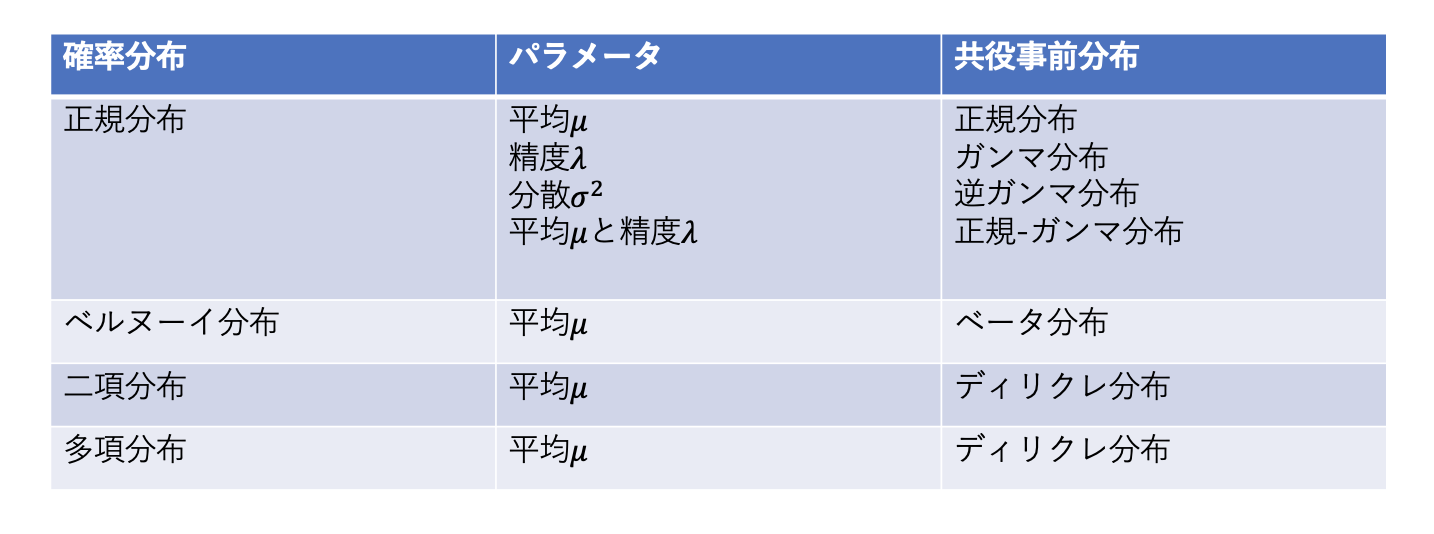
Summary of Likelihood Functions and Their Conjugate Priors
| Likelihood Function (Data Distribution) | Parameter | Conjugate Prior |
|---|---|---|
| Bernoulli distribution | Success probability \(\mu\) | Beta distribution |
| Binomial distribution | Success probability \(\mu\) | Beta distribution |
| Categorical distribution | Category probabilities \(\mu\) | Dirichlet distribution |
| Multinomial distribution | Category probabilities \(\mu\) | Dirichlet distribution |
| Normal distribution | Mean \(\mu\) | Normal distribution |
| Normal distribution | Precision \(\lambda\) | Gamma distribution |
| Normal distribution | Mean \(\mu\) , Precision \(\lambda\) | Normal-Gamma distribution |
Edge Cases and Caveats
- Relation to the uniform prior: \(\text{Beta}(1,1)\) coincides with the uniform distribution on \([0,1]\) (the Bayes–Laplace prior). \(\text{Beta}(0,0)\) (the Haldane prior), on the other hand, has a divergent integral and is an improper prior — it is not a valid probability distribution on its own. However, as long as the data contains at least one success and one failure, the posterior \(\text{Beta}(k, n-k)\) is proper.
- The pseudo-count interpretation: as the derivation above shows, the prior parameters \(a, b\) can be read as pseudo-observations of \(a-1\) successes and \(b-1\) failures assumed before seeing any data. The stronger the prior (the larger \(a, b\) are), the smaller the relative influence of the actual data (we confirm this numerically below).
- Asymptotic behavior as \(n \to \infty\) : conjugate priors give an analytically tractable posterior update, but as \(n\) grows the posterior becomes dominated by the likelihood (i.e., concentrates near the maximum-likelihood estimate) and the influence of the prior vanishes. This is a special case of the Bernstein–von Mises theorem, a general asymptotic-normality result guaranteeing that, under regularity conditions, the posterior converges to a normal distribution around the true parameter regardless of the prior chosen.
- When conjugacy is unavailable: conjugate priors only exist when the likelihood belongs to the exponential family. For example, the likelihood of logistic regression (which involves the sigmoid function) has no analytical conjugate prior; it requires either a special device such as Pólya-Gamma data augmentation (Polson, Scott & Windle, 2013) or approximate inference via variational Bayes ( Variational Bayes ) or MCMC ( Markov Chain Monte Carlo ).
Executed Python Verification
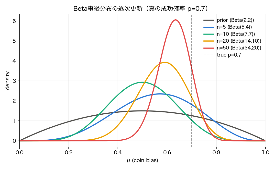
We verify Beta-Binomial conjugacy with an actual coin-flip simulation. A coin with true success probability \(p=0.7\) is flipped 50 times, and the posterior is updated sequentially starting from a \(\text{Beta}(2,2)\) prior.
import numpy as np
from scipy import stats

rng = np.random.default_rng(42)

true_p = 0.7
n_total = 50
flips = rng.binomial(1, true_p, size=n_total)

a0, b0 = 2, 2  # weakly informative prior Beta(2,2)
checkpoints = [0, 5, 10, 20, 50]
for n in checkpoints:
    k = flips[:n].sum()
    a, b = a0 + k, b0 + (n - k)
    mean = a / (a + b)
    mode = (a - 1) / (a + b - 2) if a > 1 and b > 1 else float("nan")
    lo, hi = stats.beta.ppf([0.025, 0.975], a, b)
    print(f"n={n:3d}  successes={k:3d}  posterior=Beta({a},{b})  "
          f"mean={mean:.4f}  MAP={mode:.4f}  95%CI=[{lo:.4f}, {hi:.4f}]")
The executed output is:
n=  0  successes=  0  posterior=Beta(2,2)   mean=0.5000  MAP=0.5000  95%CI=[0.0943, 0.9057]
n=  5  successes=  3  posterior=Beta(5,4)   mean=0.5556  MAP=0.5714  95%CI=[0.2449, 0.8430]
n= 10  successes=  5  posterior=Beta(7,7)   mean=0.5000  MAP=0.5000  95%CI=[0.2513, 0.7487]
n= 20  successes= 12  posterior=Beta(14,10) mean=0.5833  MAP=0.5909  95%CI=[0.3854, 0.7681]
n= 50  successes= 32  posterior=Beta(34,20) mean=0.6296  MAP=0.6346  95%CI=[0.4980, 0.7521]
As \(n\) grows, the posterior mean approaches the true value \(p=0.7\) (reaching \(0.6296\) at \(n=50\) ), and the width of the 95% credible interval shrinks monotonically from \([0.0943, 0.9057]\) (width \(0.8114\) ) to \([0.4980, 0.7521]\) (width \(0.2541\) ).
Next, we check how the “strength” of the prior affects the posterior. With \(n=8\) observations and \(k=6\) successes (a sample proportion of \(0.75\) ), we compare posterior means under priors of varying strength.
for (a0s, b0s, label) in [
    (1, 1, "Uniform Beta(1,1)"),
    (2, 2, "Weak Beta(2,2)"),
    (20, 20, "Strong Beta(20,20)"),
]:
    a, b = a0s + 6, b0s + (8 - 6)
    mean = a / (a + b)
    print(f"{label:22s} -> posterior=Beta({a},{b})  mean={mean:.4f}")
Uniform Beta(1,1)      -> posterior=Beta(7,3)   mean=0.7000
Weak Beta(2,2)         -> posterior=Beta(8,4)   mean=0.6667
Strong Beta(20,20)     -> posterior=Beta(26,22)  mean=0.5417
As the prior grows stronger (\(a_0=b_0=20\) ), the posterior mean is pulled increasingly toward the prior’s center \(0.5\) for the same data — exactly what the pseudo-count interpretation predicts (\(\text{Beta}(20,20)\) carries the same information as having already observed 20 successes and 20 failures, so it barely moves given only 8 new observations with 6 successes).
Finally, for Normal-Normal conjugacy, we generate 30 data points from a normal distribution with mean 3 and variance 4, and sequentially update from a prior \(\mathcal{N}(0, 9)\) :
rng_normal = np.random.default_rng(42)
true_mean, true_var = 3.0, 4.0
n_total = 30
data = rng_normal.normal(true_mean, np.sqrt(true_var), size=n_total)

prior_mean, prior_var = 0.0, 9.0
for n in [0, 5, 10, 30]:
    xs = data[:n]
    if n == 0:
        post_mean, post_var = prior_mean, prior_var
    else:
        prec0 = 1 / prior_var
        precl = n / true_var
        post_var = 1 / (prec0 + precl)
        post_mean = post_var * (prior_mean * prec0 + xs.sum() / true_var)
    print(f"n={n:2d}  posterior mean={post_mean:.4f}  posterior var={post_var:.4f}")
n= 0  posterior mean=0.0000  posterior var=9.0000
n= 5  posterior mean=2.3895  posterior var=0.7347
n=10  posterior mean=2.2298  posterior var=0.3830
n=30  posterior mean=2.9893  posterior var=0.1314
The posterior variance decreases monotonically from \(9.0\) to \(0.1314\) , numerically confirming the derived update rule that precisions add linearly: \(1/\tau_n^2 = 1/\tau_0^2 + n/\sigma^2\) . The posterior mean fluctuates around the true mean \(3.0\) depending on sample noise (landing at \(2.9893\) for \(n=30\) ), which is expected finite-sample variation — the theoretically guaranteed property of conjugate updating is the monotonic shrinkage of the posterior variance, not any particular trajectory of the mean.
Visualizing the sequential Beta posterior update gives:
Beyond Conjugacy: Generalized Bayesian Inference
Conjugate priors are extremely convenient computationally, but they only apply when the likelihood belongs to the exponential family. Recent research has explored Generalized Bayesian Inference for models where the likelihood itself is computationally intractable. For example, Matsubara et al. (2024) propose a generalized posterior based on a discrete Fisher divergence for discrete likelihood models whose normalizing constant is intractable, and establish conditions guaranteeing posterior consistency and asymptotic normality. This is one direction that extends Bayesian uncertainty quantification to realistic models (e.g., graphical models, spatial statistics models) where no conjugate prior is available.
References
- Taro Tezuka, Understanding Bayesian Statistics and Machine Learning , Kodansha (2017)
- Polson, N. G., Scott, J. G., & Windle, J. (2013). Bayesian Inference for Logistic Models Using Pólya–Gamma Latent Variables . Journal of the American Statistical Association, 108(504), 1339-1349.
- Matsubara, T., Knoblauch, J., Briol, F.-X., & Oates, C. J. (2024). Generalized Bayesian Inference for Discrete Intractable Likelihood . Journal of the American Statistical Association, 119(547), 2345-2355.