The EM Algorithm

The EM algorithm (Expectation-Maximization Algorithm) is an iterative algorithm for estimating the parameters of statistical models that contain latent (hidden) variables in the observed data.

For example, consider the age distribution of fitness club members. There may be two groups: people in their 20s who come for strength training and people in their 50s who come for metabolic health management, each with age distributions following a normal distribution. In this case, which group each member belongs to is a “latent variable” that cannot be directly observed.

The basic idea of the EM algorithm is to simultaneously estimate both the model parameters and the latent variables by alternating between the following two steps:

1. E-step (Expectation Step): Using the current model parameters, estimate the expected values (or probability distribution) of the latent variables from the observed data. In the above example, this involves computing the “responsibility” indicating which group each member belongs to.
2. M-step (Maximization Step): Using the expected values of the latent variables estimated in the E-step, maximize the model parameters. In the above example, this involves updating the parameters such as the mean and variance of each group’s normal distribution, using the responsibilities as weights.

By repeating this process, the estimates of the model parameters and latent variables gradually improve, and the log-likelihood eventually converges to a local maximum. This article derives why repeating these two steps improves the log-likelihood, using Jensen’s inequality, and then verifies EM numerically on a classic example distinct from GMM: the two-coin problem.

Deriving the ELBO via Jensen’s Inequality

Let \(x\) denote observed data, \(z\) the latent variable, and \(\theta\) the parameters. We want to maximize the log-likelihood \(\log p(x|\theta)\) directly, but taking the log of the marginal likelihood \(p(x|\theta) = \int p(x,z|\theta)dz\) (with the latent variable integrated out) leaves an integral inside a logarithm, which is analytically awkward.

We introduce an arbitrary probability distribution \(q(z)\) over \(z\) and rewrite the expression as an identity:

Since \(\log(\cdot)\) is a concave function, Jensen’s inequality \(\log \mathbb{E}[Y] \ge \mathbb{E}[\log Y]\) holds for any random variable \(Y>0\) . Applying it here:

This lower bound \(\mathcal{L}(q,\theta)\) is the Evidence Lower Bound (ELBO). The log-likelihood is always at least as large as the ELBO, and the gap between them can be evaluated exactly:

(substituting \(p(x,z|\theta) = p(z|x,\theta)p(x|\theta)\) and using the fact that \(\log p(x|\theta)\) does not depend on \(z\) and can be pulled out of the expectation). Because the KL divergence is always non-negative, this is an exact identity — “log-likelihood = ELBO + KL divergence” — confirming that the ELBO is indeed a lower bound on the log-likelihood. It also shows that equality holds if and only if \(KL(q(z)\|p(z|x,\theta))=0\) , i.e., \(q(z) = p(z|x,\theta)\) .

EM as Coordinate Ascent on the ELBO

This fact lets us understand the two steps of EM in a unified way: as coordinate ascent, alternately optimizing \(q\) and \(\theta\) to maximize the ELBO.

• E-step: Fix \(\theta\) at its current estimate \(\hat{\theta}\) and find the \(q(z)\) that maximizes the ELBO. From the argument above, this means setting \(q(z) = p(z|x,\hat{\theta})\) (i.e., computing the posterior itself). This makes \(KL=0\) , so \(\mathcal{L}(q,\hat{\theta}) = \log p(x|\hat{\theta})\) — the ELBO matches the log-likelihood exactly.
• M-step: Fix \(q(z)=p(z|x,\hat{\theta})\) and find the \(\theta\) that maximizes the ELBO.

Since the entropy term \(H(q)\) does not depend on \(\theta\) , maximizing the ELBO over \(\theta\) is equivalent to maximizing the Q-function \(Q(\theta,\hat{\theta}) = \mathbb{E}_{p(z|x,\hat{\theta})}[\log p(x,z|\theta)]\) — this is exactly the M-step.

After updating \(\theta\) in the M-step (assuming the Q-function improves), the ELBO also improves, but the fixed \(q(z)=p(z|x,\hat{\theta})\) is no longer the posterior under the new parameter \(\theta^{(t+1)}\) , so \(KL>0\) and the ELBO now sits strictly below the log-likelihood. However, “log-likelihood \(\ge\) ELBO” always holds, so we obtain the chain of inequalities:

which proves that the log-likelihood is monotonically non-decreasing at every EM iteration (the first inequality is “log-likelihood ≥ ELBO”, the second is the M-step improving the ELBO, and the final equality is the property right after the E-step). This general proof holds for any latent variable model, not just GMM. The GMM-specific numerical details — covariance singularities and convergence behavior — are covered in k-means and GMM: Theory, Comparison, and Python Implementation , which is worth reading alongside this article.

Gaussian Mixture Models and the EM Algorithm

The EM algorithm is commonly used for parameter estimation in Gaussian Mixture Models (GMM), which assume that observed data is generated from a superposition of multiple Gaussian distributions. Here we specialize the general argument above to GMM (the complete-data log-likelihood and its expectation being the Q-function follows directly from the previous section).

The Q Function

In the EM algorithm, the hypothetical situation where both the observed data \(x\) and the latent variables \(z\) are known is called “complete data.” We consider the log-likelihood of the joint distribution \(p(x, z | \theta)\) of the complete data.

Parameter Update Formulas for GMM via the EM Algorithm

The update formulas for estimating the parameters of a Gaussian mixture model (weights \(\pi_j\) , means \(\mu_j\) , variances \(\sigma_j^2\) of each Gaussian) using the EM algorithm are as follows:

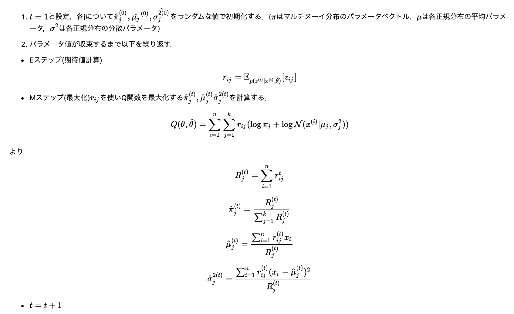
1. Initialization: Initialize the parameters \(\hat{\pi}_j^{(0)}, \hat{\mu}_j^{(0)}, \hat{\sigma}_j^{2(0)}\) of each Gaussian with random values.
2. E-step: Compute the “responsibility” \(r_{ij}\) indicating which Gaussian generated each data point \(x_i\) .

Here, \(z_{ij}=1\) indicates that data point \(x_i\) belongs to the \(j\) -th Gaussian.

3. M-step: Using the responsibilities \(r_{ij}\) computed in the E-step, calculate the new parameters \(\hat{\theta}^{(t+1)}\) .

4. Convergence check: Repeat steps 2 and 3 until the parameter changes become sufficiently small or the maximum number of iterations is reached.

A Classic Example: The Two-Coin Problem (Do & Batzoglou, 2008)

GMM works with continuous data, but the EM algorithm applies with the same reasoning to much simpler discrete settings. Here we implement the “two-coin problem,” a widely used teaching example, and inspect its convergence numerically.

Setup: There are two coins, A and B, each with an unknown probability of heads \(\theta_A, \theta_B\) . We run 5 trials, flipping a coin 10 times per trial, but which coin was used in each trial (the latent variable) was not recorded. We must estimate \(\theta_A, \theta_B\) from the observed data (the number of heads per trial) alone.

import numpy as np

# Do & Batzoglou (2008): 5 trials x 10 flips
data = np.array([
    [1,0,0,0,1,1,0,1,0,1],
    [1,1,1,1,0,1,1,1,1,1],
    [1,0,1,1,1,1,1,0,1,1],
    [1,0,1,0,0,0,1,1,0,0],
    [0,1,1,1,0,1,1,1,0,1],
])
n_heads = data.sum(axis=1)
n_tails = data.shape[1] - n_heads

def bernoulli_loglik(k, n, p):
    return k*np.log(p) + (n-k)*np.log(1-p)

def em_two_coins(n_heads, n_tails, theta_a0, theta_b0, n_iter=10):
    theta_a, theta_b = theta_a0, theta_b0
    n = n_heads + n_tails
    loglik_history = []
    for t in range(n_iter):
        # E-step: responsibility that each trial used coin A
        loglik_a = bernoulli_loglik(n_heads, n, theta_a)
        loglik_b = bernoulli_loglik(n_heads, n, theta_b)
        m = np.maximum(loglik_a, loglik_b)
        wa, wb = np.exp(loglik_a - m), np.exp(loglik_b - m)
        r_a = wa / (wa + wb)
        r_b = 1 - r_a

        # observed-data log-likelihood (coin chosen with a fair 50/50 mixture)
        mix = 0.5*np.exp(loglik_a) + 0.5*np.exp(loglik_b)
        loglik_history.append(np.log(mix).sum())

        # M-step: weighted maximum likelihood update
        theta_a = (r_a*n_heads).sum() / (r_a*n).sum()
        theta_b = (r_b*n_heads).sum() / (r_b*n).sum()
    return theta_a, theta_b, loglik_history

theta_a, theta_b, loglik_history = em_two_coins(n_heads, n_tails, 0.6, 0.5, n_iter=10)
for i, ll in enumerate(loglik_history):
    print(f"iter {i+1:2d}: log-likelihood = {ll:.6f}")
print(f"converged theta_A = {theta_a:.4f}, theta_B = {theta_b:.4f}")

The executed output is:

iter  1: log-likelihood = -33.093863
iter  2: log-likelihood = -31.859258
iter  3: log-likelihood = -31.723116
iter  4: log-likelihood = -31.627827
iter  5: log-likelihood = -31.584947
iter  6: log-likelihood = -31.573058
iter  7: log-likelihood = -31.570678
iter  8: log-likelihood = -31.570275
iter  9: log-likelihood = -31.570212
iter 10: log-likelihood = -31.570202
converged theta_A = 0.7967, theta_B = 0.5197

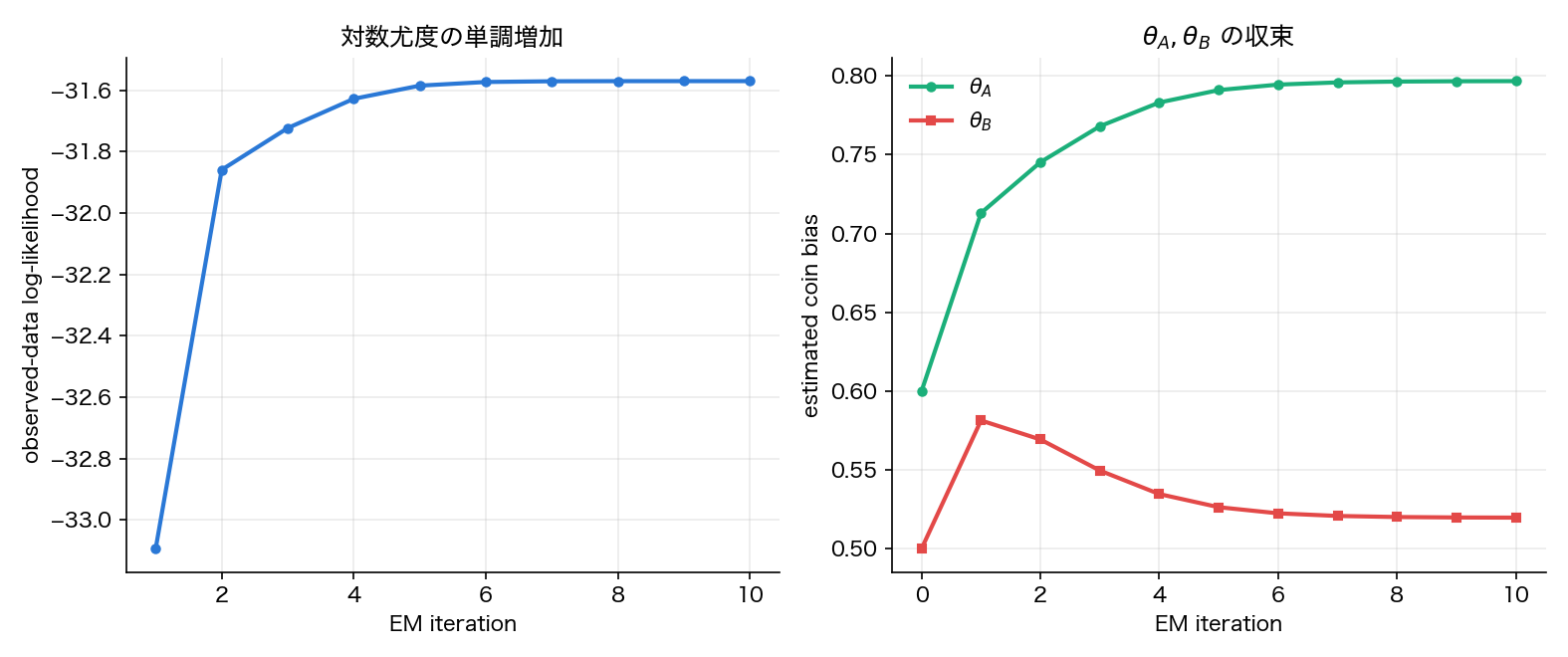
The log-likelihood increases monotonically from \(-33.09\) to \(-31.57\) , converging after 10 iterations to \(\theta_A \approx 0.797\) , \(\theta_B \approx 0.520\) — closely matching the original paper’s reported values of \(\theta_A\approx0.80\) , \(\theta_B\approx0.52\) (Do & Batzoglou, 2008). This numerically confirms the monotonic non-decrease of the log-likelihood proved above, on a discrete model quite different from GMM.

Visualizing the convergence of the log-likelihood and of \(\theta_A, \theta_B\) :

Edge Cases and Caveats

• Dependence on initialization (local optima): the only thing EM guarantees is monotonic non-decrease of the log-likelihood — not convergence to the global optimum. Running the same data with different initializations gives:

for (ia, ib) in [(0.6, 0.5), (0.5, 0.6), (0.9, 0.1), (0.5, 0.5)]:
    ta, tb, llh = em_two_coins(n_heads, n_tails, ia, ib, n_iter=15)
    print(f"init=({ia},{ib}) -> converged=({ta:.4f},{tb:.4f}), final loglik={llh[-1]:.4f}")

init=(0.6,0.5) -> converged=(0.7968,0.5196), final loglik=-31.5702
init=(0.5,0.6) -> converged=(0.5196,0.7968), final loglik=-31.5702
init=(0.9,0.1) -> converged=(0.7968,0.5196), final loglik=-31.5702
init=(0.5,0.5) -> converged=(0.6600,0.6600), final loglik=-32.0518

Initializations \((0.6,0.5)\) and \((0.5,0.6)\) converge to symmetric solutions that merely swap the labels of coins A and B (label switching: latent-variable models are generally non-identifiable up to a relabeling of components). Starting from the perfectly symmetric initialization \((0.5,0.5)\) , however, EM gets stuck at an inferior saddle-point-like solution \(\theta_A=\theta_B=0.66\) (log-likelihood \(-32.05\) ), never reaching the true optimum (log-likelihood \(-31.57\) ). In practice, the standard remedy is to run EM from multiple random initializations and keep the solution with the highest log-likelihood (multi-start).

• Convergence criteria: whether you monitor the change in parameters, in the Q-function, or in the log-likelihood affects exactly when you stop. In the example above, the change in log-likelihood drops below \(10^{-4}\) after 10 iterations.
• GMM-specific pathologies: divergence caused by a covariance matrix collapsing toward singularity (in principle the log-likelihood can diverge to \(+\infty\) ) is a GMM-specific pathology that the general argument in this article does not by itself explain. See k-means and GMM: Theory, Comparison, and Python Implementation for details.

Recent Developments in EM Convergence Theory

Analyzing the rate of EM’s convergence is a harder problem than proving monotonic non-decrease of the log-likelihood (which we derived above), and it remains an active research area. For instance, Caprio & Johansen (2025, Biometrika) propose a framework for non-asymptotically bounding the convergence rate of the EM algorithm under a logarithmic Sobolev inequality condition. Their approach views EM as coordinatewise minimization of a free-energy functional related to the KL divergence — consistent with the Jensen’s-inequality derivation in this article, and a modern extension of the same theory.

References

• Taro Tezuka, Understanding Bayesian Statistics and Machine Learning , Kodansha (2017)
• Do, C. B., & Batzoglou, S. (2008). What is the expectation maximization algorithm? Nature Biotechnology, 26(8), 897-899.
• Caprio, R., & Johansen, A. M. (2025). Fast convergence of the expectation-maximization algorithm under a logarithmic Sobolev inequality . Biometrika, 112(4).