What Is PID Control?
PID control is a type of feedback control widely used to bring the output value \(y(t)\) of a controlled system closer to the target value \(r(t)\) . It computes a control input \(u(t)\) based on the error \(e(t) = r(t) - y(t)\) between the system output and the target value, and applies it to the controlled system to achieve stabilization, improved target tracking, and disturbance rejection.
This article covers the theoretical foundations of PID control: deriving the closed-loop transfer function, analyzing steady-state error via the Final Value Theorem, and the mathematical mechanisms behind three implementation pitfalls — integral windup, derivative kick, and derivative-term noise amplification. For implementation-focused content (discretization, Ziegler-Nichols tuning, disturbance-rejection experiments), see PID Control in Python: Simulation and Tuning .
P Control (Proportional Control)
The control input \(u(t)\) in P control is determined proportionally to the error \(e(t)\) .
\[ u(t) = K_P e(t) \]- \(K_P\) : Proportional gain.
- Characteristics: Increasing \(K_P\) speeds up the response to the error and reduces it. However, making \(K_P\) too large can cause oscillatory responses and eventually make the control unstable. Also, since the control input decreases as the error decreases, a steady-state error (residual error in steady state) may remain between the output and the target value. We derive exactly why this happens in “ Analyzing Steady-State Error: The Final Value Theorem ” below.
PI Control (Proportional-Integral Control)
The control input \(u(t)\) in PI control is determined by the sum of a proportional term and an integral term.
\[ u(t) = K_P e(t) + K_I \int_0^t e(\tau)d\tau \]- \(K_I\) : Integral gain.
- Characteristics: The integral term accounts for the accumulation of past errors and therefore eliminates steady-state error. Since it continues to produce a control input until the error reaches zero, it can ultimately achieve exact tracking of the target value. However, the integral action introduces a lag in the response, which can lead to overshoot (exceeding the target value) and hunting (oscillation around the target value) in response to rapid changes.
PID Control (Proportional-Integral-Derivative Control)
The control input \(u(t)\) in PID control is determined by the sum of three components: a proportional term, an integral term, and a derivative term.
\[ u(t) = K_P e(t) + K_I \int_0^t e(\tau)d\tau + K_D \frac{de(t)}{dt} \]- \(K_D\) : Derivative gain.
- Characteristics: The derivative term predicts the trend of the error by reflecting its rate of change into the control input. This enables fast responses to rapid changes in the error, suppresses overshoot and hunting, and reduces response lag. On the other hand, the derivative term has side effects: it produces a large spike when the setpoint changes abruptly (derivative kick), and it amplifies measurement noise. Both are covered in “ Three PID Pitfalls: Derivation and Numerical Verification ” below.
PID control achieves a well-balanced control system that satisfies stability, target tracking, and responsiveness by operating based on the “present (P term),” “past (I term),” and “future (D term)” of the error. Proper tuning of the three parameters \(K_P, K_I, K_D\) is essential for PID control to function effectively.
Deriving the Closed-Loop Transfer Function
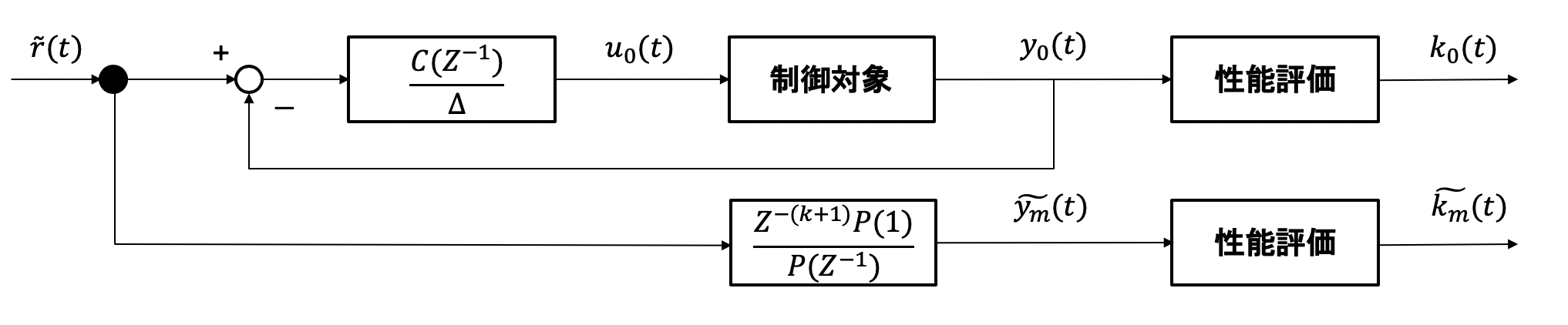
To rigorously discuss steady-state error and stability, we first derive the closed-loop transfer function. The block diagram above represents a unity-feedback loop around a plant \(G(s)\) . Let \(R(s)\) be the reference, \(Y(s)\) the output, \(E(s)\) the error, and \(U(s)\) the controller output (control input). Three relations hold:
\[ E(s) = R(s) - Y(s), \qquad U(s) = C(s)E(s), \qquad Y(s) = G(s)U(s) \]Here \(C(s)\) is the transfer function of the PID controller, obtained by taking the Laplace transform of the definition of \(u(t)\) :
\[ C(s) = K_P + \frac{K_I}{s} + K_D s = \frac{K_D s^2 + K_P s + K_I}{s} \tag{1} \]Eliminating \(Y(s)\) from the three relations gives
\[ E(s) = R(s) - G(s)C(s)E(s) \quad\Longrightarrow\quad E(s)\big(1 + G(s)C(s)\big) = R(s) \]so the transfer function from reference to error, and from reference to output, are respectively
\[ \frac{E(s)}{R(s)} = \frac{1}{1 + L(s)}, \qquad \frac{Y(s)}{R(s)} = \frac{L(s)}{1 + L(s)}, \qquad L(s) \equiv C(s)G(s) \tag{2} \]\(L(s)\) is called the open-loop transfer function — the loop gain obtained by cutting the feedback loop open. From equation (1), \(C(s)\) has a pole at \(s=0\) whenever \(K_I \ne 0\) , so \(L(s)\) inherits that pole. Whether or not \(L(s)\) has this “pole at the origin” determines the steady-state-error properties derived next.
Analyzing Steady-State Error: The Final Value Theorem
The Final Value Theorem
Let \(X(s)\) be the Laplace transform of a signal \(x(t)\) . If every pole of \(sX(s)\) lies in the open left half-plane, the Final Value Theorem (FVT) holds:
\[ \lim_{t \to \infty} x(t) = \lim_{s \to 0} sX(s) \]If this stability condition is not satisfied, the theorem cannot be applied. Assuming the closed loop is stable, we apply the FVT to \(E(s)\) from equation (2) to compute the steady-state error \(e_{ss} \equiv \lim_{t\to\infty} e(t)\) .
Steady-State Error Under P Control (a Type-0 Plant)
Consider a first-order plant \(G(s) = K/(1+Ts)\) (process gain \(K\) , time constant \(T\) ) as the controlled system. This \(G(s)\) has no pole at \(s=0\) (\(G(0)=K\) is finite and nonzero), so it is called a Type-0 plant.
Under P control, \(C(s) = K_P\) (constant), so \(L(s) = K_P G(s)\) . For a step reference \(r(t)=1 \;(t\ge0)\) , i.e. \(R(s)=1/s\) , equation (2) gives
\[ E(s) = \frac{1}{s\big(1 + K_P G(s)\big)} \]Applying the FVT,
\[ e_{ss} = \lim_{s \to 0} sE(s) = \frac{1}{1 + K_P G(0)} = \frac{1}{1 + K_P K} \tag{3} \]As long as \(K_P, K > 0\) , this value is never zero. This is the rigorous basis for “P control leaves a steady-state error.” For example, with \(K=1.0\) and \(K_P=2.0\) , \(e_{ss} = 1/(1+2) \approx 0.333\) (matching the value measured in the simulation in PID Control in Python ).
Eliminating Steady-State Error via the Integral Term: The Internal Model Principle
Under PI or PID control, \(C(s)\) has a pole at \(s=0\) as shown in equation (1). Consequently \(L(s)=C(s)G(s)\) also diverges as \(s\to0\) (as long as \(K_I \ne 0\) , \(L(s) \sim K_I K/s \to \infty\) even though \(G(0)=K\ne0\) ). Applying equation (2) to a step reference \(R(s)=1/s\) :
\[ e_{ss} = \lim_{s \to 0} s \cdot \frac{1}{s\big(1+L(s)\big)} = \lim_{s \to 0} \frac{1}{1+L(s)} = 0 \tag{4} \]Since \(L(s)\to\infty\) , \(e_{ss}\) is exactly zero. Viewed at the level of the whole closed loop, \(L(s)\) having a pole at \(s=0\) means, through the denominator \(1+L(s)\) of \(Y(s)/R(s)\) , that the closed loop passes a reference signal with a pole at the origin (a step) with zero error — this structure is called a Type-1 system.
This is a special case of the more general Internal Model Principle (Francis & Wonham, 1976): to asymptotically track a reference signal generated by some exogenous signal generator (for a step, the generator is \(1/s\) ; for a ramp, \(1/s^2\) ) with zero steady-state error, the open-loop transfer function \(L(s)\) of the control loop must internally contain the same poles as that generator. The generator for a step reference is \(1/s\) , so tracking it requires an integrator (\(1/s\) ) somewhere in the loop. A Type-0 plant has no integrator of its own, so the I term supplies it — this is the theoretical justification for “the integral term eliminates steady-state error.”
Ramp-Tracking Error: Comparing PI and PID Control
What about the steady-state error to a ramp reference \(r(t) = t\) (i.e. \(R(s) = 1/s^2\) )? From equation (2),
\[ e_{ss} = \lim_{s \to 0} s \cdot \frac{1/s^2}{1+L(s)} = \lim_{s \to 0} \frac{1}{s\big(1+L(s)\big)} \]Under PI control, \(C(s) = K_P + K_I/s = (K_P s + K_I)/s\) , so
\[ L(s) = \frac{(K_P s + K_I)K}{s(1+Ts)} \]As \(s\to0\) , \(s \cdot L(s) \to K_I K\) (define \(K_v \equiv \lim_{s\to0} sL(s)\) , the velocity error constant), so
\[ e_{ss} = \lim_{s\to0} \frac{1}{s + sL(s)} = \frac{1}{K_v} = \frac{1}{K_I K} \tag{5} \]which remains finite (nonzero). Under PID control, \(C(s) = (K_D s^2+K_P s+K_I)/s\) , but
\[ sL(s) = \frac{(K_D s^2+K_P s+K_I)K}{1+Ts} \;\xrightarrow{s\to0}\; K_I K \]and the \(K_D\) term vanishes as \(s\to0\) , so \(K_v = K_I K\) is exactly the same as for PI control. In other words, the derivative gain \(K_D\) makes no contribution whatsoever to the ramp-tracking steady-state error. What D improves is the transient response (overshoot and settling time); the only ways to reduce the steady-state error to a ramp are to increase \(K_I\) or to add an extra integrator to the plant itself.
The simulation below verifies this numerically. With \(G(s)=1/(1+s)\) (\(K=1,T=1\) ), \(K_P=2.0\) , \(K_I=1.5\) PI/PID controllers are driven with a ramp reference \(r(t)=t\) , and \(K_D\) is varied over \(0, 0.3, 0.6\) to compare the steady-state error.
import numpy as np

K_plant, T_plant = 1.0, 1.0
Kp, Ki = 2.0, 1.5

class FirstOrderSystem:
    def __init__(self, gain, time_constant, dt):
        self.gain = gain
        self.time_constant = time_constant
        self.dt = dt
        self.y = 0.0
    def update(self, u):
        self.y += self.dt / self.time_constant * (self.gain * u - self.y)
        return self.y

def simulate_ramp(kp, ki, kd, dt=0.01, t_end=60.0, ramp_rate=1.0):
    plant = FirstOrderSystem(K_plant, T_plant, dt)
    integral = 0.0
    prev_error = 0.0
    t = 0.0
    e_hist = []
    while t < t_end:
        r = ramp_rate * t
        e = r - plant.y
        integral += e * dt
        d = (e - prev_error) / dt
        prev_error = e
        u = kp * e + ki * integral + kd * d
        plant.update(u)
        e_hist.append(e)
        t += dt
    return np.array(e_hist)

for kd in [0.0, 0.3, 0.6]:
    e_hist = simulate_ramp(Kp, Ki, kd)
    e_ss_numeric = np.mean(e_hist[-200:])  # average over the last 2s
    e_ss_theory = 1.0 / (Ki * K_plant)
    print(f"Kd={kd:4.1f}: e_ss(numeric)={e_ss_numeric:.5f}, "
          f"theory 1/(Ki*K)={e_ss_theory:.5f}")
Kd= 0.0: e_ss(numeric)=0.66667, theory 1/(Ki*K)=0.66667
Kd= 0.3: e_ss(numeric)=0.66667, theory 1/(Ki*K)=0.66667
Kd= 0.6: e_ss(numeric)=0.66667, theory 1/(Ki*K)=0.66667
The numeric simulation exactly matches the theoretical value \(1/(K_I K) = 1/1.5 \approx 0.6667\) , and \(e_{ss}\) is unchanged as \(K_D\) varies.
Three PID Pitfalls: Derivation and Numerical Verification
The ideal continuous-time PID law of equation (1) is simple, but three phenomena substantially degrade performance in real implementations. Here we derive the mechanism behind each and verify the effect with a compact numerical experiment. For a more detailed comparison of countermeasures (deriving back-calculation and clamping, analyzing discretization error, etc.), see PID Control in Python .
Integral Windup
Every real actuator has a limited output range. The unsaturated control command
\[ u_{unsat}(t) = K_P e(t) + K_I \int_0^t e(\tau) d\tau + K_D \frac{de(t)}{dt} \]is in practice saturated as follows:
\[ u(t) = \begin{cases} u_{max} & (u_{unsat}(t) > u_{max}) \\ u_{unsat}(t) & (u_{min} \le u_{unsat}(t) \le u_{max}) \\ u_{min} & (u_{unsat}(t) < u_{min}) \end{cases} \]In a naive implementation, the integral state \(I(t)=\int_0^t e(\tau)d\tau\) depends only on the error \(e(t)\) and never checks whether the applied \(u(t)\) has diverged from \(u_{unsat}(t)\) due to saturation. Consequently, as long as \(e(t)\) keeps the same sign while the actuator is saturated, \(I(t)\) keeps growing without bound even though the control is not actually taking effect. This is integral windup. Once the output finally approaches the target and \(e(t)\) ’s sign flips, unwinding the excess \(I(t)\) requires integrating an opposite-sign error for a long time, during which \(u_{unsat}(t)\) stays beyond the saturation limit — resulting in large overshoot.
One standard countermeasure is conditional integration: freeze the integral only while the controller is saturated and the sign of the error is pushing further into saturation (the direction integration should be stopped); otherwise integrate as usual.
\[ \frac{dI}{dt} = \begin{cases} 0 & \big(\text{saturated and } \mathrm{sign}(e(t)) \text{ matches the saturation direction}\big) \\ e(t) & (\text{otherwise}) \end{cases} \]The simulation below compares plain PID (no anti-windup) with conditional integration. The plant is \(G(s)=1/(1+s)\) , gains are \(K_P=1.0\) , \(K_I=3.5\) , \(K_D=0.3\) , the output is limited to \(u \in [-1.15, 1.15]\) (the steady-state required input is \(u_{ss}=1.0\) ), and we compare the step response to a target \(r=1.0\) .
import numpy as np

K_plant, T_plant = 1.0, 1.0
Kp, Ki, Kd = 1.0, 3.5, 0.3
u_lo, u_hi = -1.15, 1.15
dt, t_end, setpoint = 0.01, 15.0, 1.0

class FirstOrderSystem:
    def __init__(self, gain, time_constant, dt):
        self.gain = gain
        self.time_constant = time_constant
        self.dt = dt
        self.y = 0.0
    def update(self, u):
        self.y += self.dt / self.time_constant * (self.gain * u - self.y)
        return self.y

class PIDNoAntiWindup:
    """Naive PID: the integral is always accumulated, even while saturated."""
    def __init__(self, kp, ki, kd, dt, limits):
        self.kp, self.ki, self.kd, self.dt = kp, ki, kd, dt
        self.lo, self.hi = limits
        self.integral = 0.0
        self.prev_error = None
    def update(self, setpoint, measured):
        error = setpoint - measured
        if self.prev_error is None:
            self.prev_error = error
        self.integral += error * self.dt
        p = self.kp * error
        i = self.ki * self.integral
        d = self.kd * (error - self.prev_error) / self.dt
        self.prev_error = error
        u_unsat = p + i + d
        return min(max(u_unsat, self.lo), self.hi), u_unsat

class PIDConditionalIntegration:
    """Conditional integration: freeze the integral only while the
    saturation direction matches the sign of the error."""
    def __init__(self, kp, ki, kd, dt, limits):
        self.kp, self.ki, self.kd, self.dt = kp, ki, kd, dt
        self.lo, self.hi = limits
        self.integral = 0.0
        self.prev_error = None
    def update(self, setpoint, measured):
        error = setpoint - measured
        if self.prev_error is None:
            self.prev_error = error
        p = self.kp * error
        i_tentative = self.ki * (self.integral + error * self.dt)
        d = self.kd * (error - self.prev_error) / self.dt
        self.prev_error = error
        u_unsat = p + i_tentative + d
        saturated_high = u_unsat > self.hi
        saturated_low = u_unsat < self.lo
        pushing_further = (saturated_high and error > 0) or (saturated_low and error < 0)
        if not pushing_further:
            self.integral += error * self.dt
        u = min(max(u_unsat, self.lo), self.hi)
        return u, u_unsat

def run(controller_cls, t_end, dt, setpoint_val):
    t = np.arange(0, t_end, dt)
    plant = FirstOrderSystem(K_plant, T_plant, dt)
    ctrl = controller_cls(Kp, Ki, Kd, dt, (u_lo, u_hi))
    y_hist, int_hist = [], []
    for _ in t:
        u, _ = ctrl.update(setpoint_val, plant.y)
        y = plant.update(u)
        y_hist.append(y)
        int_hist.append(ctrl.integral)
    return t, np.array(y_hist), np.array(int_hist)

results = {
    "No anti-windup": run(PIDNoAntiWindup, t_end, dt, setpoint),
    "Conditional integration": run(PIDConditionalIntegration, t_end, dt, setpoint),
}

for name, (t, y, integral) in results.items():
    overshoot = (np.max(y) - setpoint) / setpoint * 100
    tol = 0.02 * setpoint
    settle_idx = next(i for i in range(len(y)) if np.all(np.abs(y[i:] - setpoint) < tol))
    print(f"{name}: overshoot={overshoot:.2f}%, settle_t={t[settle_idx]:.2f}s, "
          f"peak_integral={np.max(integral):.4f}")
No anti-windup: overshoot=14.46%, settle_t=8.04s, peak_integral=0.7217
Conditional integration: overshoot=4.79%, settle_t=3.67s, peak_integral=0.3377
| Method | Overshoot | Settling time (within 2%) | Peak integral state |
|---|---|---|---|
| No anti-windup | 14.46% | 8.04 s | 0.7217 |
| Conditional integration | 4.79% | 3.67 s | 0.3377 |
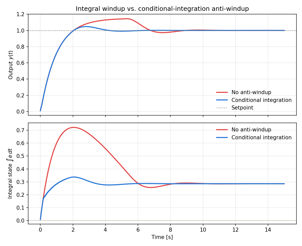
Conditional integration reduces the peak integral state by about 53%, cuts overshoot from 14.46% to 4.79%, and shortens the settling time from 8.04 s to 3.67 s. A comparison against back-calculation and clamping, along with more general discrete-time implementation details, is derived in the corresponding section of PID Control in Python .
Derivative Kick
The derivative term \(K_D \, de(t)/dt\) uses the rate of change of the error \(e(t)=r(t)-y(t)\) , which decomposes as
\[ \frac{de(t)}{dt} = \frac{dr(t)}{dt} - \frac{dy(t)}{dt} \]At the instant the reference \(r(t)\) changes as a step, the first term \(dr/dt\) is ideally a Dirac delta (in discrete time, a finite value \(\Delta r/\Delta t\) that grows arbitrarily large as \(\Delta t\) shrinks). This produces an instantaneous, large spike in the control input — the derivative kick. The standard fix is derivative-on-measurement: let the derivative term act only on the measured output \(y\) , not on the error \(e\) .
\[ d(t) = -K_D \frac{dy(t)}{dt} \]While the reference is held constant, \(de/dt = -dy/dt\) , so this form returns exactly the same value as the ordinary derivative term. In other words, it removes the kick at a setpoint change without sacrificing any disturbance-rejection or noise-response characteristics.
The simulation below compares the control input when the reference steps from \(0 \to 1\) at \(t=2\) s (\(K_P=2.5\) , \(K_I=1.2\) , \(K_D=0.6\) , \(G(s)=1/(1+s)\) ).
import numpy as np

K_plant, T_plant = 1.0, 1.0
Kp, Ki, Kd = 2.5, 1.2, 0.6
dt = 0.01

class FirstOrderSystem:
    def __init__(self, gain, time_constant, dt):
        self.gain = gain
        self.time_constant = time_constant
        self.dt = dt
        self.y = 0.0
    def update(self, u):
        self.y += self.dt / self.time_constant * (self.gain * u - self.y)
        return self.y

class PIDErrorDerivative:
    """Standard form: the derivative term acts on the error e = r - y."""
    def __init__(self, kp, ki, kd, dt):
        self.kp, self.ki, self.kd, self.dt = kp, ki, kd, dt
        self.integral = 0.0
        self.prev_error = None
    def update(self, setpoint, measured):
        error = setpoint - measured
        if self.prev_error is None:
            self.prev_error = error
        self.integral += error * self.dt
        p = self.kp * error
        i = self.ki * self.integral
        d = self.kd * (error - self.prev_error) / self.dt
        self.prev_error = error
        return p + i + d

class PIDMeasurementDerivative:
    """Derivative-on-measurement: the derivative term acts only on -y."""
    def __init__(self, kp, ki, kd, dt):
        self.kp, self.ki, self.kd, self.dt = kp, ki, kd, dt
        self.integral = 0.0
        self.prev_measured = None
    def update(self, setpoint, measured):
        error = setpoint - measured
        if self.prev_measured is None:
            self.prev_measured = measured
        self.integral += error * self.dt
        p = self.kp * error
        i = self.ki * self.integral
        d = -self.kd * (measured - self.prev_measured) / self.dt
        self.prev_measured = measured
        return p + i + d

t = np.arange(0, 8.0, dt)
step_time = 2.0
setpoint = np.where(t < step_time, 0.0, 1.0)

for name, cls in [("Derivative-on-error", PIDErrorDerivative),
                   ("Derivative-on-measurement", PIDMeasurementDerivative)]:
    pid = cls(Kp, Ki, Kd, dt)
    plant = FirstOrderSystem(K_plant, T_plant, dt)
    u_hist = []
    for sp in setpoint:
        u = pid.update(sp, plant.y)
        plant.update(u)
        u_hist.append(u)
    u_hist = np.array(u_hist)
    idx_step = np.argmax(t >= step_time)
    jump = u_hist[idx_step] - u_hist[idx_step - 1]
    print(f"{name}: u just before step={u_hist[idx_step-1]:.4f}, "
          f"u just after step={u_hist[idx_step]:.4f}, jump={jump:.4f}")
Derivative-on-error: u just before step=0.0000, u just after step=62.5120, jump=62.5120
Derivative-on-measurement: u just before step=0.0000, u just after step=2.5120, jump=2.5120
| Variant | \(u\) just before step | \(u\) just after step | Change |
|---|---|---|---|
| Derivative-on-error (standard) | 0.0000 | 62.5120 | +62.512 |
| Derivative-on-measurement | 0.0000 | 2.5120 | +2.512 |
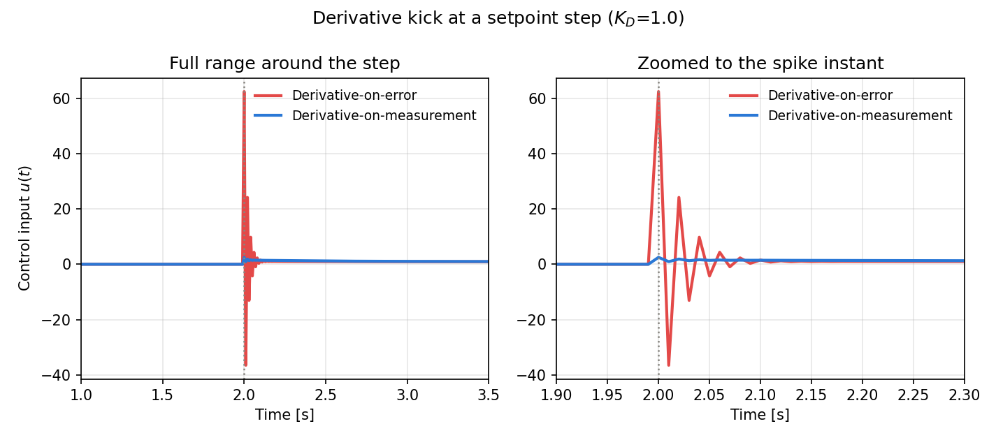
With the standard derivative term, the control input spikes to about 62.5 the instant the setpoint steps, but with derivative-on-measurement it stays around 2.51 (close to the proportional term’s jump \(K_P \Delta r = 2.5\) ). The zoomed panel in the figure also shows ringing (oscillatory decay) that follows the derivative kick. Since a spike of this size would cause mechanical shock or saturation in a real actuator, derivative-on-measurement is close to a de facto standard implementation.
Derivative-Term Noise Amplification
In the frequency domain, the derivative term has gain \(D(j\omega) = K_D \cdot j\omega\) , whose magnitude \(\lvert D(j\omega) \rvert = K_D \omega\) grows without bound, proportional to the angular frequency \(\omega\) . Measurement noise generally has content across a wide frequency band, so an ideal (unfiltered) derivative greatly amplifies high-frequency noise. The standard fix is a filtered derivative: a first-order low-pass filter attached to the derivative term.
\[ D(s) = \frac{K_D s}{1 + s/N} = \frac{K_D N s}{s + N} \]\(N\) is called the derivative filter coefficient; it sets the filter’s corner frequency (time constant \(\tau_f=1/N\) ). The frequency response is \(\lvert D(j\omega) \rvert = K_D N \omega / \sqrt{\omega^2+N^2}\) : for \(\omega \ll N\) it matches the ideal derivative, while as \(\omega \to \infty\) it saturates at \(K_D N\) , keeping high-frequency noise amplification finite.
The simulation below adds Gaussian noise with standard deviation \(0.02\) to the measured output of \(G(s)=1/(1+s)\) under PID control with \(K_P=2.5\) , \(K_I=0.8\) , \(K_D=0.6\) , and compares the steady-state (\(t>5\) s) control-input fluctuation for no filter, \(N=8\) , and \(N=1.5\) (a stronger filter).
import numpy as np

K_plant, T_plant = 1.0, 1.0
Kp, Ki, Kd = 2.5, 0.8, 0.6
dt, noise_std = 0.01, 0.02

class FirstOrderSystem:
    def __init__(self, gain, time_constant, dt):
        self.gain = gain
        self.time_constant = time_constant
        self.dt = dt
        self.y = 0.0
    def update(self, u):
        self.y += self.dt / self.time_constant * (self.gain * u - self.y)
        return self.y

class PIDFilteredDerivative:
    """Derivative-on-measurement with an optional first-order low-pass
    filter (time constant 1/N) on the raw derivative (None = no filter)."""
    def __init__(self, kp, ki, kd, dt, N=None):
        self.kp, self.ki, self.kd, self.dt = kp, ki, kd, dt
        self.N = N
        self.integral = 0.0
        self.prev_measured = None
        self.d_filt = 0.0
    def update(self, setpoint, measured):
        error = setpoint - measured
        if self.prev_measured is None:
            self.prev_measured = measured
        self.integral += error * self.dt
        p = self.kp * error
        i = self.ki * self.integral
        d_raw = -(measured - self.prev_measured) / self.dt
        self.prev_measured = measured
        if self.N is None:
            d_used = d_raw
        else:
            tau_f = 1.0 / self.N
            alpha = min(self.dt / tau_f, 1.0)
            self.d_filt += alpha * (d_raw - self.d_filt)
            d_used = self.d_filt
        return p + i + self.kd * d_used

dt_arr = np.arange(0, 15.0, dt)
setpoint = np.ones_like(dt_arr)

std_ref = None
for label, N in [("No filter", None), ("N=8", 8.0), ("N=1.5 (stronger filter)", 1.5)]:
    np.random.seed(7)
    pid = PIDFilteredDerivative(Kp, Ki, Kd, dt, N=N)
    plant = FirstOrderSystem(K_plant, T_plant, dt)
    u_hist = []
    for sp in setpoint:
        noisy_measurement = plant.y + np.random.normal(0, noise_std)
        u = pid.update(sp, noisy_measurement)
        plant.update(u)
        u_hist.append(u)
    u_hist = np.array(u_hist)
    mask = dt_arr > 5.0
    u_std = np.std(u_hist[mask])
    if std_ref is None:
        std_ref = u_std
    print(f"{label}: std(u)={u_std:.4f}, ptp(u)={np.ptp(u_hist[mask]):.4f}, "
          f"amplification_factor={u_std/std_ref:.3f}")
No filter: std(u)=2.7418, ptp(u)=19.1303, amplification_factor=1.000
N=8: std(u)=0.1476, ptp(u)=0.9491, amplification_factor=0.054
N=1.5 (stronger filter): std(u)=0.0681, ptp(u)=0.4360, amplification_factor=0.025
| Filter setting | std(u) | Peak-to-peak(u) | Ratio to unfiltered |
|---|---|---|---|
| No filter | 2.7418 | 19.1303 | 1.000 |
| \(N=8\) | 0.1476 | 0.9491 | 0.054 |
| \(N=1.5\) (stronger filter) | 0.0681 | 0.4360 | 0.025 |
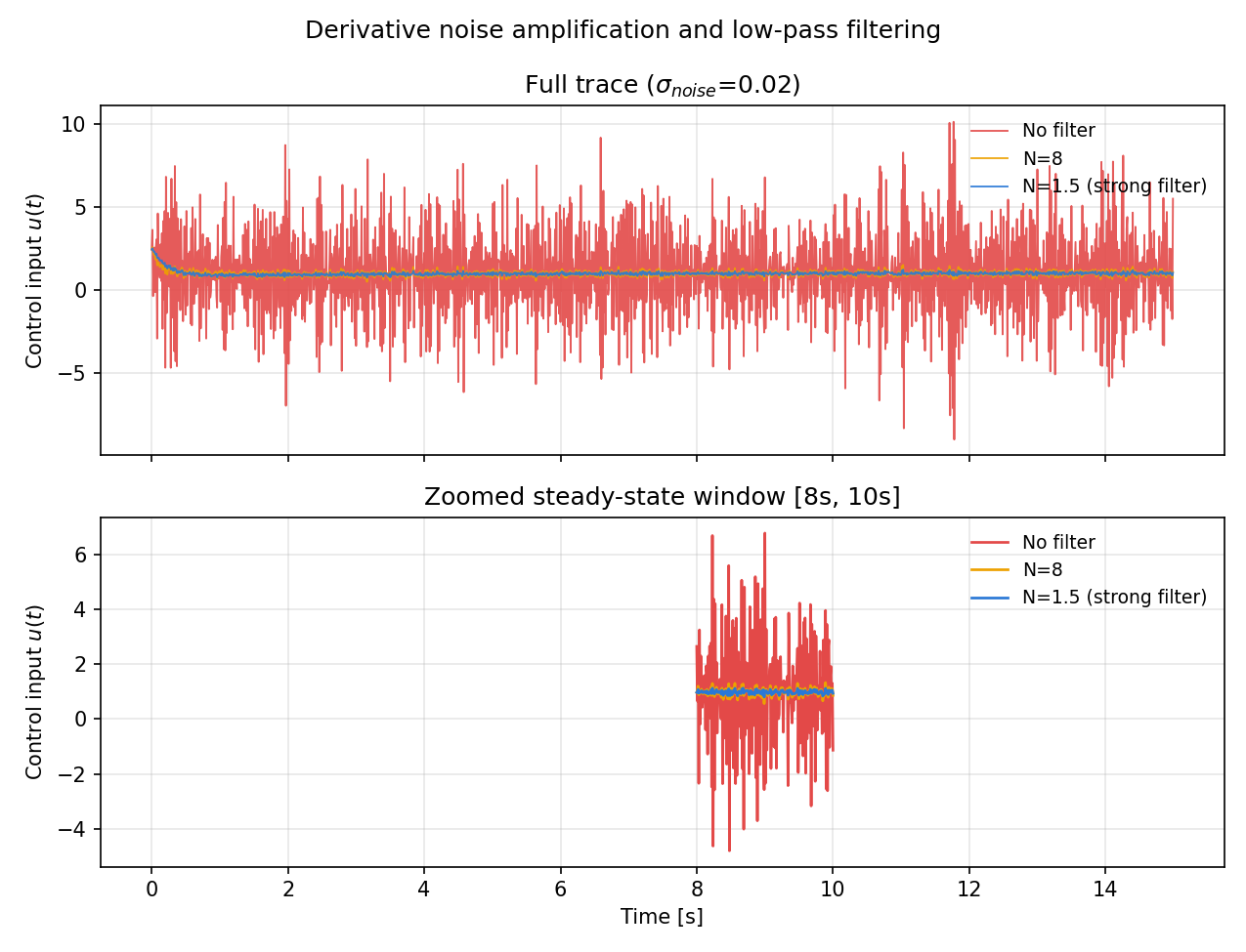
Without a filter, the control input’s standard deviation is amplified to 2.74; the \(N=8\) filter cuts this by about a factor of 18.6 (to 0.148), and strengthening the filter to \(N=1.5\) reduces it by about a factor of 40 (to 0.068). Making the filter time constant \(\tau_f=1/N\) too large relative to the plant’s response speed introduces non-negligible phase lag and erodes stability margin, so choosing \(N\) involves a genuine trade-off.
Recent Research on PID Tuning and Robustness
Classical PID control theory is a mature field, yet theoretical reinterpretation and updated implementation guidance continue to appear.
Systematizing anti-windup design: Caparroz, Soltész, Hägglund, and Guzmán (arXiv:2606.01959, 2026) compare multiple anti-windup techniques — including the back-calculation and conditional-integration methods covered in this article — across both setpoint-tracking and disturbance-rejection scenarios, and propose a new hybrid scheme combining conditional integration with dynamic back-calculation. Notably, they find experimentally that the optimal tracking time constant for back-calculation tends to be smaller than the integral time and varies substantially with saturation ratio and controller aggressiveness, giving practitioners concrete guidance for near-optimal performance without heavy computation.
Reinterpreting the Internal Model Principle: Shi (arXiv:2411.14678, 2024) reinterprets the PID controller as a combination of two mechanisms — a homogeneous controller that stabilizes the system and a disturbance observer that estimates and compensates for an unknown lumped disturbance — reinforcing, from a disturbance-compensation perspective, the role of the I term derived in this article via the Internal Model Principle. The paper also analyzes how measurement noise affects parameter selection and demonstrates applications to underactuated VTOL aircraft and lateral vehicle control.
Theoretical links between gains and robustness: Zhu, Yu, and Liu (arXiv:2504.15081, 2025) propose “PID-GM,” which reformulates the PID gains as a nonlinear mapping from three auxiliary parameters, and use singular perturbation theory to show that, for an uncertain second-order plant, closed-loop stability and steady-state-error performance are explicitly tied to a single virtual singular-perturbation parameter. Their finding that all three gains vary monotonically with this parameter offers a more systematic alternative to this article’s gain-tuning guidance (adjusting \(K_P, K_I, K_D\) individually). This field moves quickly, so please consult each paper’s primary source for specific figures and scope of applicability.
Summary
This article reviewed the three basic forms of PID control (P, PI, PID), derived the closed-loop transfer function, and used the Final Value Theorem to rigorously establish: P control’s steady-state error, how the I term eliminates it via the Internal Model Principle, and the ramp-tracking error of PI vs. PID control (showing that \(K_D\) makes no contribution). We then derived the mechanisms behind three implementation pitfalls — integral windup, derivative kick, and derivative-term noise amplification — and verified each with a numerical simulation and figure.
PID control theory is simple, but only a correct understanding of these properties makes it possible to design gains and implement anti-windup and filtering appropriately. For implementation-focused content (discretization, Ziegler-Nichols tuning, disturbance-rejection experiments), see PID Control in Python ; for evaluating stability margins, see Bode Plot or Nyquist Plot and Root Locus ; and when robustness against plant uncertainty must be guaranteed, see H-infinity Control .
References
- Astrom, K. J., & Murray, R. M. (2021). Feedback Systems: An Introduction for Scientists and Engineers (2nd ed.). Princeton University Press.
- Åström, K. J., & Hägglund, T. (1995). PID Controllers: Theory, Design, and Tuning (2nd ed.). Instrument Society of America.
- Francis, B. A., & Wonham, W. M. (1976). “The internal model principle of control theory”. Automatica, 12(5), 457-465.
- Caparroz, M., Soltész, K., Hägglund, T., & Guzmán, J. L. (2026). “Anti-Windup in PID Control: Review, Analysis, and New Tuning Directions”. arXiv:2606.01959.
- Shi, X. (2024). “Reinterpreting PID Controller From the Perspective of State Feedback and Lumped Disturbance Compensation”. arXiv:2411.14678.
- Zhu, B., Yu, W., & Liu, H. H. T. (2025). “PID-GM: PID Control with Gain Mapping”. arXiv:2504.15081.
Related Articles
- PID Control in Python: Simulation and Tuning - Implements this article’s theory in Python, with a detailed comparison of discretization methods and anti-windup schemes, plus a practical walkthrough of Ziegler-Nichols tuning.
- Bode Plot: Reading and Creating Frequency Response Diagrams with Python Implementation - Explains gain margin and phase margin, the classical stability-margin indicators — foundational for judging how far a PID gain can be raised.
- Nyquist Plot, Root Locus, and Stability Margins in Python - Uses the open-loop transfer function \(L(s)\) derived in this article to evaluate PID gain stability limits via the Nyquist criterion and root locus.
- H-infinity Control - Explains a robust-control framework that builds plant uncertainty directly into the design variables, contrasted with the PID control covered here.
- MPPI (Model Predictive Path Integral): A Unified View with the Cross-Entropy Method - Explains model predictive control based on Monte Carlo sampling, an advanced control method that goes beyond PID.
- Measuring Kubernetes’ Horizontal Pod Autoscaler (HPA) as a PID Control Loop - An applied piece that measures this article’s theme — P control’s steady-state error and its elimination — via a comparative simulation of Kubernetes’ HPA and a PID controller.