Machine Learning Terminology
In machine learning, a model is a mathematical formula or algorithm that learns from data. It contains adjustable parameters that are optimized based on given data through a process called learning or training.
A representative model is the Neural Network (NN), which mimics the neural circuits of the human brain. A multi-layered version is called a Deep Neural Network (DNN).
Learning methods are broadly divided into three categories:
- Supervised Learning
- Unsupervised Learning
- Reinforcement Learning
Overview of Reinforcement Learning
Unlike supervised and unsupervised learning where datasets are provided, reinforcement learning is characterized by being given an environment.
- Environment: A space where an agent (the learning entity) takes actions, states change according to those actions, and “rewards” are given when certain states are reached or certain actions are taken.
In reinforcement learning, the agent adjusts its model parameters to obtain more rewards through interaction with the environment. A sequence of actions and state transitions from the start to the end of the environment is called one episode, and the goal of learning is to maximize the cumulative reward obtained in one episode.
Problem Formulation: Markov Decision Process (MDP)
Reinforcement learning problems are often formulated as a Markov Decision Process (MDP). An MDP is a decision-making process with the Markov property (the next state depends only on the current state and action, not on past history).
The main components of an MDP are the following four elements:
- \(S\) : The set of States. Represents the current situation of the agent.
- \(A\) : The set of Actions. The choices available to the agent in each state.
- \(T\) : Transition Probability. The probability \(P(s'|s, a)\) of transitioning to the next state \(s'\) when taking action \(a\) in state \(s\) .
- \(R\) : Reward Function. The reward \(R(s, a, s')\) obtained when taking action \(a\) in state \(s\) and transitioning to the next state \(s'\) .
The “robot” or “AI” in reinforcement learning can be viewed as a function that receives these states and outputs optimal actions. This function is called the Policy \(\pi(a|s)\) . The agent aims to discover the optimal policy by updating its policy to maximize rewards.
There is one more essential ingredient in an MDP: the discount factor \(\gamma \in [0,1]\) . As noted above, the objective is to maximize cumulative reward, but if we simply summed all future rewards as-is, the sum could diverge for tasks that run indefinitely, and it would treat “a reward right now” and “a reward 100,000 steps from now” as equally important. \(\gamma\) discounts future rewards to present value; with it included, an MDP is formalized as the 5-tuple \((S, A, T, R, \gamma)\) . We’ll examine \(\gamma\) ’s concrete role through a numerical experiment later in this article.
Instead of keeping \(T(s'|s,a)\) (transition probability) and \(R(s,a,s')\) (reward function) separate, it is also common to combine them into the joint distribution of the next state and reward, \(p(s',r \mid s,a) = \Pr(S_{t+1}=s', R_{t+1}=r \mid S_t=s, A_t=a)\) . This more general notation also handles stochastic rewards, and is used in most references including Sutton & Barto’s textbook Reinforcement Learning: An Introduction. We use this \(p(s',r|s,a)\) notation in the derivations below; when the reward is a deterministic function of \((s,a,s')\) , it reduces to \(p(s',r|s,a) = T(s'|s,a)\) (only when \(r=R(s,a,s')\) ).
Value Functions and the Bellman Expectation Equation
The goal of reinforcement learning is to maximize cumulative reward — to handle this precisely, we define the discounted cumulative reward (return) \(G_t\) from time \(t\) onward as:
\[ G_t = R_{t+1} + \gamma R_{t+2} + \gamma^2 R_{t+3} + \cdots = \sum_{k=0}^{\infty} \gamma^k R_{t+k+1} \]From this definition, it’s immediate that \(G_t\) can be written recursively in terms of the next return \(G_{t+1}\) :
\[ G_t = R_{t+1} + \gamma \underbrace{(R_{t+2} + \gamma R_{t+3} + \cdots)}_{=\,G_{t+1}} = R_{t+1} + \gamma G_{t+1} \tag{1} \]Since the environment’s transitions are stochastic, the return \(G_t\) is itself a random variable. We therefore define the state-value function under policy \(\pi\) as the expected return:
\[ V^\pi(s) = \mathbb{E}_\pi\left[\, G_t \mid S_t = s \,\right] = \mathbb{E}_\pi\left[\sum_{k=0}^{\infty} \gamma^k R_{t+k+1} \,\middle|\, S_t = s\right] \]The Bellman Expectation Equation expresses this \(V^\pi(s)\) recursively in terms of “the value from here on,” rather than \(G_t\) directly. We substitute in equation (1) and expand.
\[ V^\pi(s) = \mathbb{E}_\pi\left[ R_{t+1} + \gamma G_{t+1} \mid S_t = s \right] \]Now we decompose the expectation over the action \(a\) chosen according to policy \(\pi(a|s)\) , and over the next state and reward \((s', r)\) arising from the joint distribution \(p(s',r|s,a)\) :
\[ V^\pi(s) = \sum_a \pi(a|s) \sum_{s',r} p(s',r|s,a) \Big[\, r + \gamma\, \mathbb{E}_\pi\big[G_{t+1} \mid S_{t+1}=s'\big] \Big] \]This is where the Markov property does the essential work. Since \(G_{t+1}\) is determined solely by transitions from time \(t+1\) onward, once \(S_{t+1}=s'\) is given, information about the earlier \(S_t=s\) or \(A_t=a\) becomes irrelevant. That is:
\[ \mathbb{E}_\pi\big[G_{t+1} \mid S_{t+1}=s', S_t=s, A_t=a\big] = \mathbb{E}_\pi\big[G_{t+1} \mid S_{t+1}=s'\big] = V^\pi(s') \]Substituting this in gives us the Bellman Expectation Equation:
\[ \boxed{\, V^\pi(s) = \sum_a \pi(a|s) \sum_{s',r} p(s',r|s,a) \big[\, r + \gamma V^\pi(s') \,\big] \,} \tag{2} \]Similarly, the action-value function \(Q^\pi(s,a) = \mathbb{E}_\pi[G_t \mid S_t=s, A_t=a]\) , representing the value of taking action \(a\) in state \(s\) , can be derived by exactly the same procedure (substituting equation (1), then simplifying the conditional expectation via the Markov property):
\[ Q^\pi(s,a) = \sum_{s',r} p(s',r|s,a) \big[\, r + \gamma\, \mathbb{E}_\pi[G_{t+1}\mid S_{t+1}=s'] \,\big] = \sum_{s',r} p(s',r|s,a) \big[\, r + \gamma V^\pi(s') \,\big] \tag{3} \]Furthermore, since \(V^\pi(s)\) is “the expected return from following \(\pi\) starting at \(s\) ,” it can be written simply by taking the expectation of \(Q^\pi\) over actions \(a \sim \pi(\cdot|s)\) :
\[ V^\pi(s) = \sum_a \pi(a|s)\, Q^\pi(s,a) \tag{4} \]Combining equations (3) and (4) recovers equation (2). \(V^\pi\) and \(Q^\pi\) are two sides of the same coin — each can be reconstructed from the other.
The Bellman Optimality Equation
The goal of reinforcement learning is to find an optimal policy \(\pi^*\) that maximizes \(V^\pi(s)\) for every state \(s\) . The value functions under the optimal policy are called the optimal state-value function \(V^*(s) = \max_\pi V^\pi(s)\) and the optimal action-value function \(Q^*(s,a) = \max_\pi Q^\pi(s,a)\) .
Here we invoke Bellman’s Principle of Optimality: “if you follow an optimal policy, no matter what your first action is, the subsequent decisions must be optimal for the remaining subproblem.” This means that after taking action \(a\) in state \(s\) , it is always best to continue following the optimal policy from then on. Therefore:
\[ Q^*(s,a) = \sum_{s',r} p(s',r|s,a) \big[\, r + \gamma V^*(s') \,\big] \tag{5} \]holds (this is just equation (3) with \(V^\pi\) replaced by \(V^*\) ). Moreover, since the optimal policy simply greedily chooses the action that maximizes \(Q^*(s,a)\) in each state:
\[ V^*(s) = \max_a Q^*(s,a) \]Substituting equation (5) gives the Bellman Optimality Equation:
\[ \boxed{\, V^*(s) = \max_a \sum_{s',r} p(s',r|s,a) \big[\, r + \gamma V^*(s') \,\big] \,} \tag{6} \]The only difference from the expectation equation (2) is that the policy-weighted average \(\sum_a \pi(a|s)(\cdots)\) has been replaced by \(\max_a(\cdots)\) . This single change is enormously important: once \(V^*\) is computed, the optimal policy is obtained directly as the greedy policy:
\[ \pi^*(s) = \arg\max_a Q^*(s,a) = \arg\max_a \sum_{s',r} p(s',r|s,a) \big[\, r + \gamma V^*(s') \,\big] \]In other words, the Bellman Optimality Equation is simultaneously “a system of \(|S|\) simultaneous equations that must hold across all states” and, provided \(\gamma < 1\) and rewards are bounded, a contraction mapping guaranteed to have a unique solution \(V^*\) . In the next section we implement two algorithms that exploit this property to iteratively compute \(V^*\) .
Solving with Dynamic Programming: A Gridworld Experiment
To verify the theory concretely, we set up a 5x5 gridworld where the environment model \(p(s',r|s,a)\) is fully known, and implement and run both Value Iteration and Policy Iteration in Python.
row/col   0     1     2     3     4
 0     .     .     .     .    G2(+10)
 1     .    WALL   .     .     .
 2     .     .   TRAP(-10) .   .
 3     .     .     .     .     .
 4    START  G1(+5) .    .     .
- Each cell is a state \(s\) ; actions are the four cardinal directions (deterministic transitions; hitting a wall or the boundary leaves the agent in place)
- Moving to a regular cell gives reward \(-1\) (a “living cost”)
- Goals
G1(nearby, small reward \(+5\) ) andG2(far, large reward \(+10\) ), andTRAP(\(-10\) ), are absorbing states where the episode ends immediately upon arrival (\(V=0\) fixed) WALLis an impassable obstacle
This setup is exactly the special case where \(p(s',r|s,a)\) is a deterministic distribution (a single \((s',r)\) occurs with probability 1), so the sums in equations (2) and (6) collapse to a single term, letting us translate the derivation directly into code.
GRID_H, GRID_W = 5, 5
G1, G2, TRAP, WALL = (4, 1), (0, 4), (2, 2), (1, 1)
TERMINALS = {G1, G2, TRAP}
REWARD = {G1: 5.0, G2: 10.0, TRAP: -10.0}
STEP_COST = -1.0
ACTIONS = ['up', 'down', 'left', 'right']
DELTA = {'up': (-1, 0), 'down': (1, 0), 'left': (0, -1), 'right': (0, 1)}

states = [(r, c) for r in range(GRID_H) for c in range(GRID_W) if (r, c) != WALL]
nonterminal_states = [s for s in states if s not in TERMINALS]

def step(s, a):
    dr, dc = DELTA[a]
    nr, nc = s[0] + dr, s[1] + dc
    if not (0 <= nr < GRID_H and 0 <= nc < GRID_W) or (nr, nc) == WALL:
        nr, nc = s  # stay in place if hitting a wall or boundary
    ns = (nr, nc)
    r = REWARD.get(ns, STEP_COST)
    return ns, r

def q_value(s, a, V, gamma):
    ns, r = step(s, a)
    v_ns = 0.0 if ns in TERMINALS else V[ns]
    return r + gamma * v_ns
Value Iteration
We use equation (6) directly as the update rule.
\[ V_{k+1}(s) \leftarrow \max_a \sum_{s',r} p(s',r|s,a) \big[\, r + \gamma V_k(s') \,\big] \]def value_iteration(gamma, theta=1e-8, max_iter=10000):
V = {s: 0.0 for s in states}
deltas = []
for it in range(1, max_iter + 1):
delta = 0.0
newV = dict(V)
for s in nonterminal_states:
newV[s] = max(q_value(s, a, V, gamma) for a in ACTIONS)
delta = max(delta, abs(newV[s] - V[s]))
V = newV
deltas.append(delta)
if delta < theta:
break
policy = {s: max(ACTIONS, key=lambda a: q_value(s, a, V, gamma))
for s in nonterminal_states}
return V, policy, it, deltas
Running this with \(\gamma=0.9\) and convergence tolerance \(\theta=10^{-8}\) (\(\max_s |V_{k+1}(s)-V_k(s)| < \theta\) ) gives:
Value Iteration: converged in 6 sweeps
delta per sweep: [10.0, 9.0, 8.1, 7.29, 2.187, 0.0]
It converged exactly (delta hits exactly 0) in 6 sweeps. The delta shrinking geometrically (roughly by a factor of \(\gamma\) each step) is a direct manifestation of the Bellman operator being a contraction mapping.
Policy Iteration
Policy iteration alternates between policy evaluation (iterating equation (2) under a fixed policy to a fixed point) and policy improvement (greedifying with respect to \(Q^\pi\) ).
def policy_evaluation(policy, gamma, theta=1e-8, max_iter=10000):
    V = {s: 0.0 for s in states}
    for sweep in range(1, max_iter + 1):
        delta = 0.0
        newV = dict(V)
        for s in nonterminal_states:
            newV[s] = q_value(s, policy[s], V, gamma)
            delta = max(delta, abs(newV[s] - V[s]))
        V = newV
        if delta < theta:
            break
    return V, sweep

def policy_iteration(gamma, theta=1e-8):
    policy = {s: 'right' for s in nonterminal_states}  # initial policy: "right" everywhere
    total_eval_sweeps, improve_iters = 0, 0
    while True:
        V, sweeps = policy_evaluation(policy, gamma, theta)
        total_eval_sweeps += sweeps
        improve_iters += 1
        new_policy, stable = {}, True
        for s in nonterminal_states:
            best_a = max(ACTIONS, key=lambda a: q_value(s, a, V, gamma))
            new_policy[s] = best_a
            if best_a != policy[s]:
                stable = False
        policy = new_policy
        if stable:
            return V, policy, improve_iters, total_eval_sweeps
Running this with the same \(\gamma=0.9\) and initial policy “right everywhere” gives:
Policy Iteration: converged after 3 policy improvements
Policy evaluation breakdown (sweeps): [176, 7, 6]  (189 sweeps total)
Only 3 policy-improvement steps were needed, but the breakdown shows the first policy evaluation alone took 176 sweeps. Under the initial “right everywhere” policy, there are states that keep bouncing off the right edge of the grid, endlessly collecting \(-1\) (never reaching an absorbing state); its value converges to \(V^\pi(s) \approx -1/(1-\gamma) = -10\) , which, at the \(\gamma=0.9\) contraction rate, takes on the order of 176 iterations. After policy improvement, the 2nd and 3rd evaluations converge rapidly (7 and 6 sweeps) because every state now follows a “sensible” policy that reaches a terminal state in at most about 8 steps.
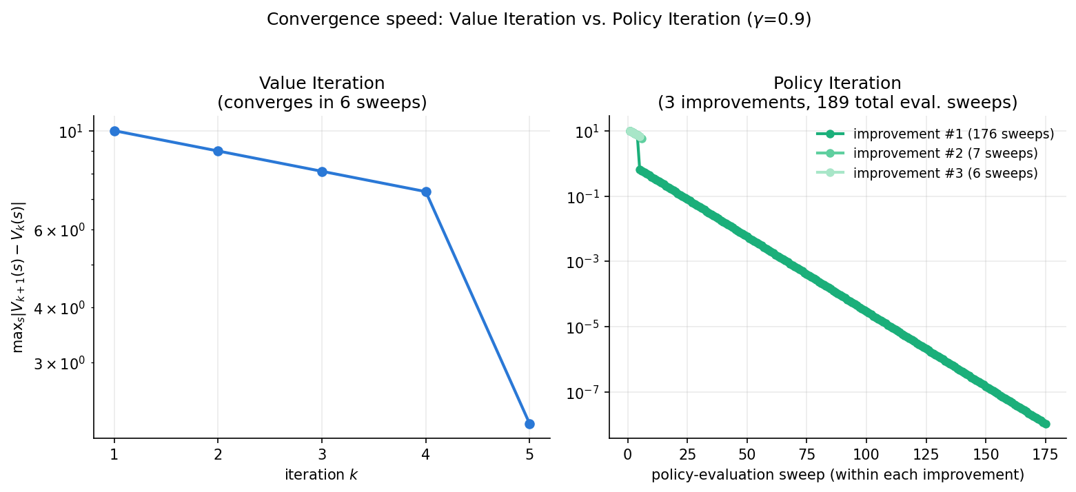
This result illustrates the classic trade-off between the two methods. Value iteration does a cheap update each sweep (just a max over actions per state), but needs repeated sweeps to converge to \(V^*\) (6 sweeps here). Policy iteration needs few improvement steps (3 here), but each improvement step requires solving policy evaluation to convergence, and the total work (189 sweeps) turned out larger than value iteration’s in this case. Which is more efficient depends on the problem (number of states, quality of the initial policy, the policy-evaluation stopping criterion, etc.).
Cross-Verification: Do Both Converge to the Same Optimum?
We check that these two independent algorithms arrive at the same answer.
V_vi, pi_vi, _, _ = value_iteration(0.9)
V_pi, pi_pi, _, _ = policy_iteration(0.9)

max_diff = max(abs(V_vi[s] - V_pi[s]) for s in nonterminal_states)
policy_match = all(pi_vi[s] == pi_pi[s] for s in nonterminal_states)
print(max_diff, policy_match)
# => 0.0  True
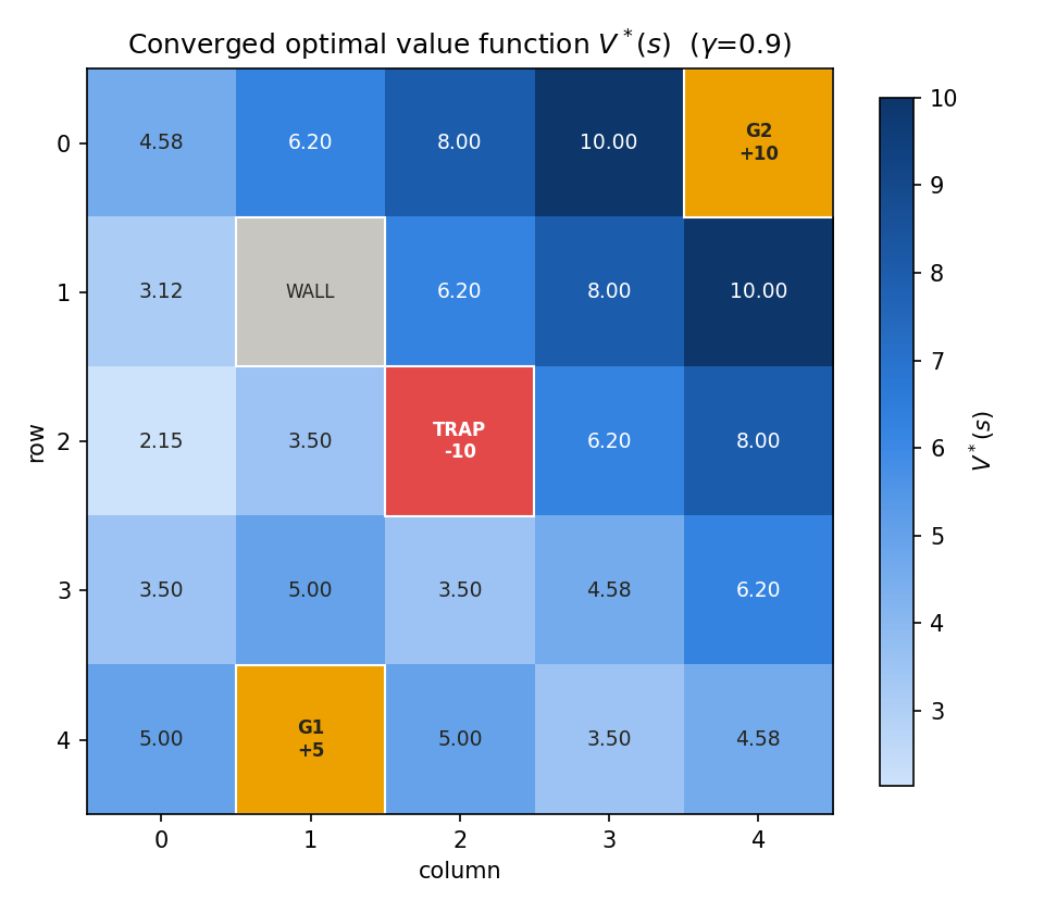
The maximum difference is exactly 0.0, and the optimal policy matches exactly across all 21 states. Value iteration and policy iteration are completely different procedures as algorithms, but since both are solving the same fixed-point equation — the Bellman Optimality Equation (6) — theory guarantees that if they converge, they converge to the same \(V^*\) and \(\pi^*\) . This experiment confirms it numerically.
Visualizing the converged \(V^*(s)\) as a heatmap makes it immediately clear that value is higher near the goals and lower near the trap.
The Role of the Discount Factor γ: Near Reward vs. Far Reward
We now verify concretely that \(\gamma\)
controls “how much the agent cares about the future.” This gridworld deliberately places both a nearby, small reward G1 (\(+5\)
, one cell from the start) and a distant, large reward G2 (\(+10\)
, Manhattan distance 8 cells). We run value iteration with \(\gamma = 0.5\)
, \(0.9\)
, and \(0.99\)
, and tally which goal the optimal policy from each state heads toward.
def terminal_reached(policy, s, max_steps=100):
    cur = s
    for _ in range(max_steps):
        if cur in TERMINALS:
            return cur
        cur, _ = step(cur, policy[cur])
    return None

for g in [0.5, 0.9, 0.99]:
    _, pi_g, _, _ = value_iteration(g)
    c1 = sum(terminal_reached(pi_g, s) == G1 for s in nonterminal_states)
    c2 = sum(terminal_reached(pi_g, s) == G2 for s in nonterminal_states)
    print(f"gamma={g}: states heading to G1={c1}, states heading to G2={c2}")
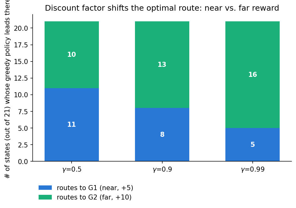
gamma=0.5:  states heading to G1=11, states heading to G2=10
gamma=0.9:  states heading to G1=8,  states heading to G2=13
gamma=0.99: states heading to G1=5,  states heading to G2=16
Out of 21 states, the number choosing the distant, larger reward G2 goes 10 → 13 → 16 monotonically as \(\gamma\)
increases. A myopic agent (small \(\gamma\)
) tends to jump at the nearby G1, while a far-sighted agent (\(\gamma\)
close to 1) is willing to go the long way around for the bigger G2.
Focusing on a single state makes this switch even more concrete. At state \((1,0)\) (bottom-left of the wall), the optimal value and optimal action change as follows:
| \(\gamma\) | \(V^*((1,0))\) | Optimal action | Heads to |
|---|---|---|---|
| 0.5 | \(-1.125\) | down | nearby G1 |
| 0.9 | \(3.122\) | up | distant G2 |
| 0.99 | \(5.666\) | up | distant G2 |
At \(\gamma=0.5\)
, the path toward G1 has higher value, so the optimal action is “down”; at \(\gamma=0.9\)
and above, the discounted value of the path toward G2 overtakes it, and the optimal action flips to “up.” This experiment shows that changing a single hyperparameter, \(\gamma\)
, can change the optimal policy itself, even with the same environment and the same reward design.
Toward Model-Free Reinforcement Learning
The value iteration and policy iteration covered so far are both dynamic programming methods that assume the joint distribution of transitions and rewards, \(p(s',r|s,a)\) , is fully known. In practice, this environment model is usually unknown. The next article covers model-free reinforcement learning methods such as Q-learning and SARSA, which estimate \(Q\) purely from the agent’s actual experience (sequences of states, actions, and rewards) without a model.
Related Articles
- A Comprehensive Overview of Reinforcement Learning - A map of reinforcement learning methods and their relationships
- Model-Based Reinforcement Learning - Reinforcement learning approaches that leverage environment models
- Reinforcement Learning for ROBOTIS OP3 Walking: ROS Package Implementation - A practical application of reinforcement learning to real robots
References
- Takahiro Kubo, Introduction to Reinforcement Learning with Python , Shoeisha (2019)