The Cross-Entropy Method (CEM) is a type of importance sampling in Monte Carlo methods, used as an algorithm for optimization problems and rare event probability estimation.
Monte Carlo Sampling
The Monte Carlo method is a general term for numerical computation techniques that use random numbers to find approximate solutions to complex problems.
For example, suppose we want to find the expected value \(l = \mathbb{E}[H(X)] = \int H(x)f(x)dx\) of a function \(H(X)\) , where random variable \(X\) follows probability density function \(f(x)\) . In Monte Carlo sampling, this expected value is approximated using \(N\) independent and identically distributed samples \(X_1, \dots, X_N\) :
\[ l_{MS} = \frac{1}{N} \sum_{i=1}^{N} H(X_i) \]Importance Sampling
In Monte Carlo sampling, samples are generated directly from the probability distribution \(f(x)\) for which we want to compute the expected value. However, if the region where \(H(x)\) takes large values falls in a low-probability region of \(f(x)\) , efficient sampling becomes difficult.
In importance sampling, instead of sampling from the target distribution \(f(x)\) , samples are generated from a different sampling distribution \(g(x)\) . The expected value is then estimated by multiplying those samples by weights \(w(x) = f(x)/g(x)\) .
\[ l_{IS} = \frac{1}{N} \sum_{i=1}^N H(X_i) \frac{f(X_i)}{g(X_i)} = \mathbb{E}_g\lbrace H(X)\frac{f(X)}{g(X)}\rbrace \]Here, \(X_i \sim g(x)\) . The efficiency of importance sampling depends heavily on the choice of sampling distribution \(g(x)\) . In particular, the optimal sampling distribution \(g^*(x)\) that minimizes variance is known to take the form \(g^*(x) \propto |H(x)|f(x)\) . Below we derive this fact rigorously from the variance formula, and see how CEM is a procedure for approaching this \(g^*(x)\) .
Deriving the variance of the importance sampling estimator
Since \(l_{IS}\) is the average of \(N\) i.i.d. samples, its variance is the per-sample variance divided by \(N\) :
\[ \mathrm{Var}_g[l_{IS}] = \frac{1}{N}\left( \mathbb{E}_g\left[H(X)^2 \frac{f(X)^2}{g(X)^2}\right] - l^2 \right) \]Rewriting the expectation \(\mathbb{E}_g[\cdot]\) as an integral over \(g(x)\) ,
\[ \mathbb{E}_g\left[H(X)^2 \frac{f(X)^2}{g(X)^2}\right] = \int H(x)^2 \frac{f(x)^2}{g(x)^2}\, g(x)\,dx = \int \frac{H(x)^2 f(x)^2}{g(x)}\,dx \]Since \(l^2\) is a constant independent of \(g\) , minimizing the variance reduces to the following constrained minimization problem:
\[ \min_{g} \int \frac{H(x)^2 f(x)^2}{g(x)}\,dx \quad \text{s.t.} \quad \int g(x)\,dx = 1 \]Introducing a Lagrange multiplier \(\lambda\) and taking the functional derivative with respect to \(g(x)\) , setting it to zero,
\[ -\frac{H(x)^2 f(x)^2}{g(x)^2} + \lambda = 0 \;\Longrightarrow\; g(x)^2 = \frac{H(x)^2 f(x)^2}{\lambda} \;\Longrightarrow\; g(x) \propto |H(x)|\, f(x) \]which is exactly the form of the optimal sampling distribution \(g^*(x)\) stated above. In particular, when \(H(x) \geq 0\) everywhere (e.g. when \(H\) is an indicator function for a probability), setting the normalizing constant to \(l = \mathbb{E}_f[H(X)]\) gives \(g^*(x) = H(x)f(x)/l\) , in which case
\[ H(x)\frac{f(x)}{g^*(x)} = H(x)\frac{f(x)}{H(x)f(x)/l} = l \]is a constant \(l\) independent of \(x\) . Since a constant has zero variance, \(\mathrm{Var}_{g^*}[l_{IS}] = 0\) holds. That is, the ideal importance sampling distribution \(g^*\) gives the true expectation with zero variance — but since the definition of \(g^*\) itself contains the unknown \(l\) , it cannot be used directly. CEM is an algorithm that iteratively searches for a distribution close to this \(g^*\) within a tractable parametric family \(g(x;v)\) .
From rare-event probability estimation to optimization
CEM was originally proposed to estimate the rare-event probability \(l = \mathbb{E}_f[\mathbb{1}\{S(X)\geq\gamma\}] = P_f(S(X)\geq\gamma)\) that some function \(S(x)\) exceeds a threshold \(\gamma\) , where \(H(x) = \mathbb{1}\{S(x)\geq\gamma\}\) . The larger \(\gamma\) is, the rarer the event, and plain Monte Carlo sampling produces almost no occurrences of the event among \(N\) samples, causing the relative error (standard deviation / estimate) of the estimator to blow up. Importance sampling, by concentrating probability mass on the region where the event is likely under \(g(x;v)\) , allows stable estimation of \(l\) even with few samples.
The transition to optimization is achieved by changing the role of the threshold \(\gamma\) . In rare-event estimation, \(\gamma\) was a fixed constant; in optimization, \(\gamma_t\) is determined adaptively at each iteration as the top-\(\rho\) quantile of the samples. By repeatedly updating \(\gamma_t\) to “the best value found so far,” the sampling distribution \(g(x;v_t)\) is gradually pushed toward the neighborhood of the objective’s optimum. In other words, the optimization version of CEM can be seen not as targeting a fixed rare event, but as a sequential update of the importance sampling distribution against a moving target (the adaptive elite threshold). The next section derives how this “distribution update using an elite threshold” is formalized as cross-entropy minimization.
Cross-Entropy Method (CEM)
The Cross-Entropy Method is an algorithm for iteratively finding a distribution close to the optimal sampling distribution \(g^*(x)\) in importance sampling.
“Cross-entropy” is a measure of similarity between two probability distributions \(p\) and \(q\) , defined as:
\[ H(p, q) = -\int p(x) \log q(x) dx \]From the relationship \(KL(p||q) = \int p(x) \log \frac{p(x)}{q(x)} dx = H(p,q) - H(p)\) , when the true distribution \(p\) is fixed, minimizing the KL divergence is equivalent to minimizing the cross-entropy.
CEM optimizes the parameters \(v\) of a parameterized sampling distribution \(g(x;v)\) through the following procedure:
- Initialization: Initialize parameter \(v\) and set up the sampling distribution \(g(x;v)\) .
- Sampling: Generate \(N\) samples \(X_1, \dots, X_N\) from the current sampling distribution \(g(x;v)\) .
- Evaluation: Compute the objective function \(H(X_i)\) for each sample \(X_i\) .
- Elite Sample Selection: Select the top \(P\) percent of samples with the highest (or lowest, depending on the optimization direction) objective function values as “elite samples.”
- Parameter Update: Update the parameters \(v\) of the sampling distribution \(g(x;v)\) using the elite samples. This update maximizes the likelihood of the elite samples, which is equivalent to minimizing the cross-entropy between the empirical distribution of elite samples and \(g(x;v)\) .
- Convergence Check: Repeat from step 2 until the change in parameter \(v\) is sufficiently small or the maximum number of iterations is reached.
Through this iterative process, the sampling distribution \(g(x;v)\) gradually concentrates on the region of the optimal solution, enabling efficient search.
Deriving the elite-quantile distribution update
Steps 4-5 above — “select elite samples and update the parameters using their mean and variance” — may look ad hoc, but they can in fact be derived rigorously as the solution to a cross-entropy minimization problem.
Define the target distribution as the current sampling distribution \(g(x;v_{t-1})\) multiplied by an indicator function for the elite set, \(\mathbb{1}\{H(x) \geq \gamma_t\}\) (or \(\mathbb{1}\{H(x) \leq \gamma_t\}\) for minimization), then normalized:
\[ g^*_{\gamma_t}(x) \;\propto\; \mathbb{1}\{H(x)\geq \gamma_t\}\; g(x; v_{t-1}) \]CEM finds the \(v\) that minimizes the cross-entropy between \(g^*_{\gamma_t}\) and the parametric family \(g(x;v)\) (equivalent to KL-divergence minimization when \(p\) is fixed, as noted above):
\[ v_t = \arg\min_v D_{KL}\left(g^*_{\gamma_t} \,\|\, g(\cdot\,;v)\right) = \arg\max_v \int g^*_{\gamma_t}(x) \log g(x;v)\,dx \]Since \(g^*_{\gamma_t}\) is supported on \(g(x;v_{t-1})\) (it is just \(g(x;v_{t-1})\) multiplied by an indicator), this integral can be rewritten as an expectation over \(X \sim g(\cdot;v_{t-1})\) , and approximated by its empirical (Monte Carlo) version over the current sample set:
\[ v_t \approx \arg\max_v \frac{1}{N}\sum_{i=1}^N \mathbb{1}\{H(X_i)\geq \gamma_t\}\, \log g(X_i;v), \qquad X_i \sim g(\cdot\,;v_{t-1}) \]The samples for which \(\mathbb{1}\{H(X_i)\geq\gamma_t\} = 1\) are exactly the “elite samples,” so this maximization is nothing but maximizing the log-likelihood of the elite samples — i.e. maximum likelihood estimation (MLE) over the elite set.
Taking \(g(x;v) = \mathcal{N}(x;\mu,\Sigma)\) as a diagonal-covariance Gaussian family, the log-likelihood over the elite set \(\mathcal{E} = \{X_i : H(X_i)\geq\gamma_t\}\) (with \(n_{elite}\) elements) is
\[ \sum_{i\in\mathcal{E}} \log \mathcal{N}(X_i;\mu,\Sigma) = -\frac{n_{elite}}{2}\log|2\pi\Sigma| - \frac{1}{2}\sum_{i\in\mathcal{E}}(X_i-\mu)^\top \Sigma^{-1}(X_i-\mu) \]Differentiating with respect to \(\mu\) and \(\Sigma\) and setting to zero gives the standard Gaussian MLE result:
\[ \mu_t = \frac{1}{n_{elite}}\sum_{i\in\mathcal{E}} X_i, \qquad \Sigma_t = \frac{1}{n_{elite}}\sum_{i\in\mathcal{E}} (X_i-\mu_t)(X_i-\mu_t)^\top \]This corresponds exactly to mean = np.mean(elite_samples, axis=0) and std = np.std(elite_samples, axis=0) in the implementation shown below. In other words, the seemingly naive operation “update using the mean and variance of the elite samples” is rigorously justified as cross-entropy minimization = maximum likelihood estimation of a Gaussian over the elite set.
Note that using \(X_i \sim g(\cdot;v_{t-1})\) directly as the proposal — without explicitly applying the likelihood-ratio weight \(f(x)/g(x;v_{t-1})\) (i.e. treating it as \(=1\) ) — is a simplification of the standard CEM formulation. A fully general form that strictly follows the importance sampling framework of the previous section (using explicit likelihood-ratio weights) also exists, but in practice this simplification works well enough.
Comparison of CEM and MPPI
A closely related method to CEM is MPPI (Model Predictive Path Integral) . Both are optimization methods based on importance sampling, but they differ in how they weight samples.
| Property | CEM | MPPI |
|---|---|---|
| Weighting | Hard selection (top \(P\) % elite samples) | Soft weighting (exponential weights based on cost) |
| Update rule | Update distribution with mean/variance of elites | Update distribution with weighted mean of all samples |
| Information usage | Discards information from non-elite samples | Utilizes information from all samples |
| Temperature | None | Yes (\(\lambda\) controls sharpness of weights) |
| Application | General-purpose optimization | Primarily model predictive control (MPC) |
CEM’s operation of “selecting the top \(P\) %” corresponds to the limit \(\lambda \to 0\) of MPPI’s temperature parameter. In other words, CEM can be understood as a special case of MPPI.
Practical guidelines for choosing between them:
- Discrete optimization and combinatorial optimization are better suited for CEM
- Continuous control problems and robotics are better suited for MPPI
- MPPI has higher sample efficiency (since it uses information from all samples), but requires tuning the temperature parameter
Python Implementation of CEM
Here we present a Python implementation of the Cross-Entropy Method for solving a continuous optimization problem. We use the Rastrigin function as a test function, which has many local minima.
Rastrigin Function
The Rastrigin function is a widely used benchmark for optimization algorithms, defined as:
\[ f(\mathbf{x}) = An + \sum_{i=1}^{n} \left[ x_i^2 - A\cos(2\pi x_i) \right] \]where \(A = 10\) and \(n\) is the dimensionality. The global minimum is at \(\mathbf{x}^* = \mathbf{0}\) with \(f(\mathbf{0}) = 0\) . Due to its many local minima, simple gradient-based methods struggle to find the global minimum, making it ideal for demonstrating the effectiveness of stochastic search methods like CEM.
Implementation
import numpy as np
import matplotlib.pyplot as plt

# --- Define the Rastrigin function ---
def rastrigin(x):
    """Rastrigin function (minimization target)"""
    A = 10
    return A * len(x) + np.sum(x**2 - A * np.cos(2 * np.pi * x))

# --- Cross-Entropy Method implementation ---
def cross_entropy_method(
    objective_fn,   # Objective function (to minimize)
    dim,            # Dimensionality of search space
    n_samples=100,  # Number of samples per iteration
    elite_frac=0.2, # Fraction of elite samples
    n_iterations=50,# Maximum number of iterations
    initial_mean=None,  # Initial mean
    initial_std=5.0,    # Initial standard deviation
):
    """Minimize using the Cross-Entropy Method"""

    # Step 1: Initialization
    mean = initial_mean if initial_mean is not None else np.zeros(dim)
    std = np.full(dim, initial_std)
    n_elite = int(n_samples * elite_frac)

    # History tracking
    best_scores = []      # Best score per iteration
    mean_history = []     # Mean trajectory

    for iteration in range(n_iterations):
        # Step 2: Sampling (from normal distribution)
        samples = np.random.normal(
            loc=mean, scale=std, size=(n_samples, dim)
        )

        # Step 3: Evaluation (compute objective for each sample)
        scores = np.array([objective_fn(s) for s in samples])

        # Step 4: Elite sample selection (top P% with lowest scores)
        elite_indices = np.argsort(scores)[:n_elite]
        elite_samples = samples[elite_indices]

        # Step 5: Parameter update (mean and std of elite samples)
        mean = np.mean(elite_samples, axis=0)
        std = np.std(elite_samples, axis=0)

        # Record history
        best_scores.append(np.min(scores))
        mean_history.append(mean.copy())

        # Convergence check (stop if std is small enough)
        if np.all(std < 1e-6):
            print(f"Converged at iteration {iteration + 1}.")
            break

    return mean, best_scores, mean_history

# --- Run CEM ---
np.random.seed(42)
dim = 2  # 2D problem

best_solution, best_scores, mean_history = cross_entropy_method(
    objective_fn=rastrigin,
    dim=dim,
    n_samples=200,
    elite_frac=0.1,
    n_iterations=100,
    initial_mean=np.array([3.0, -3.0]),  # Start far from optimum
    initial_std=3.0,
)

print(f"Optimal solution: {best_solution}")
print(f"Objective value: {rastrigin(best_solution):.6f}")

# --- Visualization ---
fig, axes = plt.subplots(1, 2, figsize=(14, 5))

# (a) Convergence plot
axes[0].plot(best_scores, linewidth=2)
axes[0].set_xlabel("Iteration")
axes[0].set_ylabel("Best Score")
axes[0].set_title("Convergence of CEM")
axes[0].set_yscale("log")
axes[0].grid(True, alpha=0.3)

# (b) Contour plot with search trajectory
x_grid = np.linspace(-5, 5, 200)
y_grid = np.linspace(-5, 5, 200)
X, Y = np.meshgrid(x_grid, y_grid)
Z = np.array([
    [rastrigin(np.array([xi, yi])) for xi in x_grid]
    for yi in y_grid
])

axes[1].contourf(X, Y, Z, levels=30, cmap="viridis", alpha=0.8)
axes[1].colorbar = plt.colorbar(axes[1].contourf(X, Y, Z, levels=30, cmap="viridis", alpha=0.8), ax=axes[1])

# Plot mean trajectory
mean_arr = np.array(mean_history)
axes[1].plot(mean_arr[:, 0], mean_arr[:, 1], "r.-", markersize=8, linewidth=1.5, label="Mean trajectory")
axes[1].plot(mean_arr[0, 0], mean_arr[0, 1], "rs", markersize=12, label="Start")
axes[1].plot(mean_arr[-1, 0], mean_arr[-1, 1], "r*", markersize=15, label="Final")
axes[1].plot(0, 0, "wx", markersize=12, markeredgewidth=3, label="Global optimum")
axes[1].set_xlabel("$x_1$")
axes[1].set_ylabel("$x_2$")
axes[1].set_title("CEM Search Trajectory on Rastrigin Function")
axes[1].legend(loc="upper right")

plt.tight_layout()
plt.savefig("cem_result.png", dpi=150, bbox_inches="tight")
plt.show()
Running this code demonstrates the following:
- Convergence behavior: The objective function value rapidly decreases with each iteration, approaching the global minimum \(f(\mathbf{0}) = 0\)
- Search trajectory: The mean of the sampling distribution moves from the initial point \((3, -3)\) toward the origin \((0, 0)\)
- Avoiding local minima: CEM successfully avoids the many local minima of the Rastrigin function to reach the global minimum
Key hyperparameters and their effects:
n_samples(sample count): More samples provide more stable search but increase computational costelite_frac(elite fraction): A smaller fraction increases selection pressure and speeds convergence, but risks premature convergenceinitial_std(initial standard deviation): A larger value explores a wider region but takes longer to converge
Choosing the elite fraction: convergence speed vs. diversity trade-off
As noted above, the elite quantile \(\rho\)
(elite_frac) is the single most important hyperparameter, directly trading off CEM’s convergence speed against exploration diversity. A smaller \(\rho\)
produces stronger selection pressure and faster distribution collapse, but if the collapse is too fast, the standard deviation can shrink to near zero around a local minimum too early (premature convergence), risking a failure to find the global optimum. A larger \(\rho\)
mixes in information from worse samples when computing the mean/variance, slowing the collapse and requiring more iterations.
To measure this effect, we used the 10-dimensional Rastrigin function (which has many local minima, making the impact of premature convergence pronounced). We kept the sample count small at n_samples=100 (a somewhat sample-starved condition relative to the dimensionality, where selection-pressure effects show up clearly), and for each elite quantile \(\rho \in \{0.02, 0.05, 0.1, 0.2, 0.3, 0.5\}\)
ran 30 random seeds, measuring the average number of iterations to convergence and the rate of “premature convergence” — defined as the final objective value exceeding \(5.0\)
(i.e. failing to reach the basin of the global optimum and getting stuck at a local minimum).
import numpy as np

def rastrigin(x):
    A = 10
    return A * len(x) + np.sum(x**2 - A * np.cos(2 * np.pi * x))

def cem_diag(dim, n_samples, elite_frac, n_iterations, initial_mean, initial_std, seed):
    """CEM with diagonal covariance and a convergence check; reused for KL tracking below."""
    rng = np.random.default_rng(seed)
    mean = initial_mean.copy()
    std = np.full(dim, initial_std)
    n_elite = max(1, int(n_samples * elite_frac))

    best_scores = []
    for it in range(n_iterations):
        samples = rng.normal(loc=mean, scale=std, size=(n_samples, dim))
        scores = np.array([rastrigin(s) for s in samples])
        elite_idx = np.argsort(scores)[:n_elite]
        elite = samples[elite_idx]

        mean = np.mean(elite, axis=0)
        std = np.maximum(np.std(elite, axis=0), 1e-12)

        best_scores.append(np.min(scores))
        if np.all(std < 1e-6):
            break

    return {"mean": mean, "n_iter_used": len(best_scores), "final_score": rastrigin(mean)}

elite_fracs = [0.02, 0.05, 0.1, 0.2, 0.3, 0.5]
n_seeds = 30
for ef in elite_fracs:
    iters, finals, stuck = [], [], 0
    for seed in range(n_seeds):
        res = cem_diag(
            dim=10, n_samples=100, elite_frac=ef, n_iterations=200,
            initial_mean=np.full(10, 3.0), initial_std=3.0, seed=seed,
        )
        iters.append(res["n_iter_used"])
        finals.append(res["final_score"])
        if res["final_score"] > 5.0:
            stuck += 1
    print(f"elite_frac={ef:.2f}: mean_iters={np.mean(iters):.1f} "
          f"median_final={np.median(finals):.2f} stuck(>5.0)={stuck}/{n_seeds}")
The results were as follows.
| \(\rho\) | Mean iterations | Median final score | Premature convergence rate (>5.0) |
|---|---|---|---|
| 0.02 | 18.7 | 44.33 | 30/30 (100%) |
| 0.05 | 50.0 | 14.06 | 30/30 (100%) |
| 0.10 | 73.7 | 6.97 | 18/30 (60%) |
| 0.20 | 84.9 | 3.18 | 5/30 (17%) |
| 0.30 | 85.8 | 2.99 | 6/30 (20%) |
| 0.50 | 125.1 | 2.98 | 1/30 (3%) |
With \(\rho=0.02\) , convergence is fastest at an average of 18.7 iterations, but all 30 seeds (100%) got stuck at a local minimum. As \(\rho\) increases, the premature-convergence rate drops (to 3% at \(\rho=0.5\) ), but the number of iterations needed grows to 125.1 — about 6.7x the compute cost of \(\rho=0.02\) .
Panel (a) below shows the convergence curve (log scale) for a representative seed. \(\rho=0.02\) (red line) plateaus after about 20 iterations and “locks in” to a local minimum, while \(\rho=0.5\) (blue line) continues descending more gradually but reaches a much lower value.
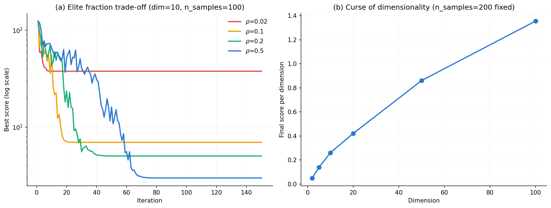
In practice, \(\rho \in [0.1, 0.2]\) is a commonly used balance between speed and reliability, but for more multimodal objectives (many local minima), a larger \(\rho\) or multi-start restarts from several initial points are recommended.
Curse of dimensionality in high dimensions
CEM’s parameter update, if the full covariance matrix \(\Sigma\) is estimated, has a number of elements that grows as \(O(d^2)\) in the dimension \(d\) (or \(O(d)\) if restricted to the diagonal, as in this article’s implementation). Estimating the covariance accurately requires scaling the sample count \(N\) with dimensionality — this is the essence of the “curse of dimensionality” that degrades CEM’s sample efficiency in high-dimensional spaces.
We measured this in practice by fixing n_samples=200 and varying the dimensionality, recording the objective value after 100 iterations (normalized per dimension as a “score per dimension”), averaged over 10 seeds (the code is the same cem_diag from the previous section called with different dim values, so it is omitted here).
| Dimension | Final score (mean) | Score per dimension | Covariance params (full) | Covariance params (diagonal) |
|---|---|---|---|---|
| 2 | 0.099 | 0.0497 | 3 | 2 |
| 5 | 0.697 | 0.1393 | 15 | 5 |
| 10 | 2.603 | 0.2603 | 55 | 10 |
| 20 | 8.409 | 0.4204 | 210 | 20 |
| 50 | 43.031 | 0.8606 | 1275 | 50 |
| 100 | 135.545 | 1.3555 | 5050 | 100 |
The per-dimension score grows roughly linearly with dimensionality (from 0.05 at 2D to 1.36 at 100D — about a 27x increase), confirming that with the same sample count and iteration budget, search becomes relatively insufficient at higher dimensions. Panel (b) above shows this trend.
We also measured how much the sample count must grow to compensate. We searched for the minimum sample count (from {50, 100, 200, 400, 800, 1600, 3200}) needed to reach a fixed target of “per-dimension score below 0.5,” averaged over 5 seeds:
| Dimension | Samples needed |
|---|---|
| 2 | 100 |
| 5 | 100 |
| 10 | 200 |
| 20 | 200 |
| 50 | 400 |
As dimensionality grows 25x (from 2 to 50), the sample count needed to hit the target grows only 4x (from 100 to 400). For CEM variants that estimate a full covariance matrix by MLE each iteration, the sample count needed for a well-conditioned estimate is theoretically known to grow on the order of \(d^2\) ; compared to that, this diagonal-covariance implementation degrades much more gently. Still, the loss of sample efficiency is not negligible.
Practical mitigations include:
- Restricting to a diagonal covariance (as in this article’s implementation, updating each dimension independently and ignoring cross-dimensional correlations) reduces the parameter count from \(O(d^2)\) to \(O(d)\) and is a standard technique for making CEM more robust in high dimensions.
- Scaling the sample count with dimensionality (a rough rule of thumb sometimes cited is \(N \gtrsim 4d\) ).
- Setting a lower bound (regularization) on the covariance to prevent search from becoming skewed when a particular dimension’s variance collapses before the others.
- For problems with strong correlations, a diagonal restriction lacks expressive power, so intermediate representations such as a low-rank covariance approximation (e.g. \(\Sigma = \sigma^2 I + UU^\top\) ) are also used as extensions.
Measuring KL divergence across distribution updates
As we saw in “Deriving the elite-quantile distribution update,” each CEM iteration is an operation that minimizes cross-entropy (KL divergence). So how does the KL divergence between the pre- and post-update distributions actually evolve across iterations? The KL divergence between two diagonal-covariance multivariate Gaussians has the following closed form:
\[ D_{KL}\!\left(\mathcal{N}(\mu_0,\Sigma_0)\,\|\,\mathcal{N}(\mu_1,\Sigma_1)\right) = \frac{1}{2}\left[ \mathrm{tr}(\Sigma_1^{-1}\Sigma_0) + (\mu_1-\mu_0)^\top \Sigma_1^{-1} (\mu_1-\mu_0) - d + \log\frac{|\Sigma_1|}{|\Sigma_0|} \right] \](where \(d\) is the dimensionality; since the matrices are diagonal, \(\mathrm{tr}\) and \(|\cdot|\) can be computed as elementwise sums/products.)
import numpy as np

def rastrigin(x):
    A = 10
    return A * len(x) + np.sum(x**2 - A * np.cos(2 * np.pi * x))

def cem_with_kl(dim, n_samples, elite_frac, n_iterations, initial_mean, initial_std, seed):
    rng = np.random.default_rng(seed)
    mean = initial_mean.copy()
    std = np.full(dim, initial_std)
    n_elite = max(1, int(n_samples * elite_frac))
    stds, kl_trace = [], []

    for it in range(n_iterations):
        samples = rng.normal(loc=mean, scale=std, size=(n_samples, dim))
        scores = np.array([rastrigin(s) for s in samples])
        elite_idx = np.argsort(scores)[:n_elite]
        elite = samples[elite_idx]

        new_mean = np.mean(elite, axis=0)
        new_std = np.maximum(np.std(elite, axis=0), 1e-12)

        var0, var1 = std**2, new_std**2
        kl = 0.5 * np.sum(var0 / var1 + (new_mean - mean) ** 2 / var1 - 1 + np.log(var1 / var0))
        kl_trace.append(kl)

        mean, std = new_mean, new_std
        stds.append(np.mean(std))
        if np.all(std < 1e-6):
            break

    return stds, kl_trace

stds, kl_trace = cem_with_kl(
    dim=2, n_samples=200, elite_frac=0.2, n_iterations=100,
    initial_mean=np.array([3.0, -3.0]), initial_std=3.0, seed=42,
)
print(f"Iterations to convergence: {len(kl_trace)}")
print(f"KL at iterations 1-5: {[round(k, 3) for k in kl_trace[:5]]}")
print(f"Max KL: {max(kl_trace):.3f} (iteration {np.argmax(kl_trace)+1})")
print(f"Final iteration KL: {kl_trace[-1]:.3f}")
Running this with the 2D Rastrigin function, n_samples=200, and elite_frac=0.2 (essentially the same settings as this article’s implementation, only elite_frac differs), convergence occurs at iteration 26, with the following trace observed:
- Iterations 1-5: \(1.431 \to 0.586 \to 0.202 \to 0.033 \to 0.151\) — a roughly decreasing trend with noise
- Starting around iteration 13, it rises again, peaking at \(11.114\) at iteration 18
- At iteration 26 (convergence), it is \(4.619\)
Intuitively, one would expect the KL divergence to monotonically decrease as the distribution converges to the optimum, but the measured result is the opposite: the KL divergence actually spikes near the end of convergence. The cause is that in this final phase, the standard deviation \(\sigma\) becomes very small in absolute terms (0.388 at iteration 12, 0.0028 at iteration 18, \(2.8\times10^{-5}\) at iteration 22), yet the relative shrinkage rate between iterations (\(\sigma_t/\sigma_{t-1}\) ) remains large until the very end. The \(\log(\Sigma_1/\Sigma_0)\) term in the KL divergence depends on the ratio of variances, so even a tiny absolute shrinkage can produce a large KL value if the ratio is large.
This is an important practical caveat: the intuition “small KL divergence implies convergence is near” does not hold during CEM’s final phase, when the distribution’s collapse is accelerating. Using an absolute threshold on the standard deviation for the convergence check (as in this article’s implementation, std < 1e-6) is more stable than relying on the KL divergence.
Recent research directions (2023 onward)
CEM has long been known as a technique for combinatorial optimization and rare-event simulation, but in recent years it has increasingly been revisited in the context of model-based reinforcement learning and model predictive control (MPC).
- Action planning in model-based reinforcement learning: Rolling out multiple action sequences under a learned dynamics model, then repeatedly evaluating, selecting elites, and resampling with CEM to decide the action sequence to execute, remains one of the standard approaches to action planning in model-based RL.
- MPC initialization and trajectory optimization: Sampling-based MPC methods, including MPPI discussed in this article, have seen exploration of hybrid update rules that combine CEM’s hard elite selection with MPPI’s soft weighting (e.g. soft weighting applied only within the top quantile), with applications to real-time trajectory optimization in robotics.
- Connections to offline reinforcement learning and safe policy search: In settings where policies are learned only from previously collected offline data, using a learned value function or dynamics model as the objective for CEM-style sampling-based optimization has been explored as a way to improve performance while constraining deviation into out-of-distribution actions.
Much of this research directly builds on the basic principle derived in this article — “distribution update via elite-quantile cross-entropy minimization” — while combining it with neural-network value functions or dynamics models. That said, this area continues to develop actively, so readers are encouraged to consult primary sources for specific method names and performance figures.
Related Articles
- Bayesian Optimization: Fundamentals and Python Implementation - Another black-box optimization approach that uses Gaussian process surrogate models instead of sampling-based search.
- MPPI (Model Predictive Path Integral): A Unified View with the Cross-Entropy Method - Extends CEM’s importance sampling framework to stochastic optimal control, with a unified mathematical perspective.
- Genetic Algorithms: Fundamentals and Python Implementation - Selection/crossover/mutation as an alternative population-based metaheuristic to CEM’s elite-based distribution update.
- Simulated Annealing: Theory and Python Implementation - Single-solution stochastic search; useful contrast with CEM’s distribution-based approach.
- Particle Swarm Optimization (PSO): Theory and Python Implementation - Swarm-intelligence-based optimizer; PSO updates velocity/position whereas CEM updates a probability distribution.
- Gaussian Process Regression: Theory and Python Implementation - The surrogate model behind Bayesian optimization, contrasting with CEM in sample efficiency.
- Markov Chain Monte Carlo (MCMC): Metropolis-Hastings and Gibbs Sampling - Counterpart Monte Carlo strategy that samples from posteriors rather than updating a parametric distribution.
- From SGD to Adam: Evolution of Gradient-Based Optimization - Gradient-based counterpart to gradient-free CEM; useful contrast for problem regime selection.
- Monte Carlo Optimization Methods Comparison (CEM/SA/GA/MPPI/PSO) - Hub article comparing five Monte Carlo optimizers including CEM under a common sample/evaluate/update skeleton, with a method-selection guide.
References
- Rubinstein, R. Y., & Kroese, D. P. (2013). The Cross-Entropy Method: A Unified Approach to Combinatorial Optimization, Monte-Carlo Simulation, and Machine Learning. Springer Science & Business Media.
- Urushihara, T., “Application of Large Deviation Theory to Importance Sampling in Monte Carlo Simulation”