H-infinity control is one of the robust control theories, a controller design method aimed at guaranteeing control performance against disturbances and model uncertainties in a system. In particular, it aims to minimize the system’s response to the worst-case disturbance.
Classical control (such as
PID control
or
stability margins from gain/phase margin
) designs a controller against a single fixed plant model and only checks robustness after the fact via stability margins. H-infinity control is fundamentally different: it builds the plant’s uncertainty directly into the design variables and solves an optimization problem that guarantees performance over the entire assumed set of uncertainties. This article works through the theoretical pillars — the small gain theorem, the H-infinity norm, the standard H-infinity control problem, and the existence conditions from the algebraic Riccati equation — deriving as much as practical, and finishes with a numerical experiment using python-control’s SLICOT-based hinfsyn, measuring how its robustness compares against PID control.
H-infinity Norm
Definition
Given the closed-loop transfer function \(T_{zw}(s)\) from disturbance \(w\) to the evaluation output \(z\) , the H-infinity norm is defined as the supremum over frequency of the largest singular value of the frequency response.
\[ \|T_{zw}\|_\infty = \sup_{\omega \in \mathbb{R}} \bar\sigma\big(T_{zw}(j\omega)\big) \]Here \(\bar\sigma(\cdot)\) denotes the largest singular value of a matrix. For SISO (single-input single-output) systems, \(\bar\sigma(T_{zw}(j\omega)) = |T_{zw}(j\omega)|\) , so the H-infinity norm is simply the peak value of the Bode magnitude curve — the gain at the worst-case frequency.
Why It Represents the “Worst-Case Gain”: The Induced L2 Norm
The H-infinity norm has another face: it is the supremum of the signal energy ratio.
\[ \|z\|_2^2 = \int_0^\infty z^T(t) z(t)\, dt, \qquad \|w\|_2^2 = \int_0^\infty w^T(t) w(t)\, dt \]Defining the L2 norm (signal energy) this way, the following identity holds for a stable system \(T_{zw}\) :
\[ \|T_{zw}\|_\infty = \sup_{w \in L_2,\, w \neq 0} \frac{\|z\|_2}{\|w\|_2} \]This claims that “the H-infinity norm is the induced norm for finite-energy inputs,” which can look like it’s asserted without proof, so let’s trace the key steps.
Upper bound (\(\leq\) ): By Parseval’s theorem, energy in the time domain is preserved as energy in the frequency domain.
\[ \|z\|_2^2 = \frac{1}{2\pi}\int_{-\infty}^{\infty} \|\hat Z(j\omega)\|^2 d\omega = \frac{1}{2\pi}\int_{-\infty}^{\infty} \|T_{zw}(j\omega)\hat W(j\omega)\|^2 d\omega \]By the definition of the largest singular value, \(\|T_{zw}(j\omega) v\| \leq \bar\sigma(T_{zw}(j\omega))\|v\|\) holds for any vector \(v\) , so
\[ \|z\|_2^2 \leq \frac{1}{2\pi}\int_{-\infty}^{\infty} \bar\sigma(T_{zw}(j\omega))^2 \|\hat W(j\omega)\|^2 d\omega \leq \|T_{zw}\|_\infty^2 \cdot \frac{1}{2\pi}\int_{-\infty}^{\infty} \|\hat W(j\omega)\|^2 d\omega = \|T_{zw}\|_\infty^2 \|w\|_2^2 \]Therefore \(\|z\|_2/\|w\|_2 \leq \|T_{zw}\|_\infty\) holds for any \(w\) .
Lower bound (\(\geq\) , achievability): Let \(\omega_0 = \arg\sup_\omega \bar\sigma(T_{zw}(j\omega))\) be the peak frequency, and consider an input aligned with the right singular vector direction \(v_0\) corresponding to the largest singular value of \(T_{zw}(j\omega_0)\) . Constructing \(w(t)\) as a narrowband signal of bandwidth \(\varepsilon\) centered at \(\omega_0\) (in direction \(v_0\) ), continuity of \(T_{zw}\) means that within the band \(\bar\sigma(T_{zw}(j\omega)) \approx \bar\sigma(T_{zw}(j\omega_0))\) , so the output-to-input energy ratio converges to \(\bar\sigma(T_{zw}(j\omega_0)) = \|T_{zw}\|_\infty\) as \(\varepsilon \to 0\) .
The upper and lower bounds coincide, giving \(\sup_w \|z\|_2/\|w\|_2 = \|T_{zw}\|_\infty\) . In other words, the H-infinity norm is the gain obtained by choosing the direction and frequency, among all finite-energy disturbances, that maximizes amplification of the output — this is why it is called the “worst-case gain.”
Numerical Verification
Let’s verify this identity directly. Take the lightly damped second-order system \(G(s) = \dfrac{1}{s^2+0.4s+4}\) (natural frequency \(\omega_n=2\,\mathrm{rad/s}\) , damping ratio \(\zeta=0.1\) ) as an example, and compute its H-infinity norm two ways.
import numpy as np
import control as ct

G = ct.tf([1.0], [1, 0.4, 4])
norm_inf, wpeak = ct.linfnorm(G)
print(f"control.linfnorm: ||G||inf = {norm_inf:.6f} at w = {wpeak:.4f} rad/s")

w = np.logspace(-2, 3, 200000)
mag = np.abs(G(1j*w))
print(f"brute force sup: max|G(jw)| = {mag.max():.6f} at w = {w[np.argmax(mag)]:.4f} rad/s")
The output was:
control.linfnorm: ||G||inf = 1.256297 at w = 1.9799 rad/s
brute force sup: max|G(jw)| = 1.256297 at w = 1.9799 rad/s
python-control’s internal algorithm (an exact solver iterating on a state-space eigenvalue problem, rather than a maximum over a frequency grid) and the brute-force frequency sweep agree to 6 decimal places. The peak frequency \(\omega=1.98\,\mathrm{rad/s}\)
is also nearly identical to the resonance frequency \(\omega_n=2\)
, matching the intuition for a lightly damped system.
Objective of the H-infinity Control Problem
The goal of the H-infinity control problem is to design a controller \(K\) that keeps the H-infinity norm \(\|T_{zw}\|_\infty\) below a positive constant \(\gamma\) .
\[ \|T_{zw}\|_\infty < \gamma \]Finding a controller that satisfies this is the objective; \(\gamma\) is called the performance index, and a smaller value indicates better disturbance rejection performance. From a game-theoretic perspective, it can be expressed as the following minimax problem.
\[ \min_u \max_w \int_0^\infty \big(z^T(t)z(t) - \gamma^2 w^T(t)w(t)\big)\, dt \]The control input \(u\) tries to minimize \(z^Tz\) , while the worst-case disturbance \(w\) tries to maximize \(w^Tw\) — this zero-sum game between \(u\) and \(w\) and its saddle point is the starting point for the Riccati-equation derivation later in this article.
Small Gain Theorem
The theoretical foundation that lets H-infinity control guarantee robustness is the Small Gain Theorem.
Setup
Suppose a stable nominal system \(M(s)\) and a stable but otherwise unknown uncertainty \(\Delta(s)\) form a feedback loop as follows.
\[ y = Mu, \qquad u = w + \Delta y \]This is the standard \(M\) –\(\Delta\) structure, where an additive perturbation \(\Delta y\) arising from the uncertainty is added to an external input \(w\) . Solving for \(u\) ,
\[ u = w + \Delta M u \;\; \Longrightarrow \;\; (I - \Delta M) u = w \;\; \Longrightarrow \;\; u = (I - \Delta M)^{-1} w \]We consider the condition under which this feedback loop is internally stable.
Theorem and Proof
Small Gain Theorem: If \(M\) and \(\Delta\) are both stable (no poles in the right half-plane) and
\[ \|M\|_\infty \, \|\Delta\|_\infty < 1 \]holds, then the closed loop \((I-\Delta M)^{-1}\) is internally stable for any such \(\Delta\) .
Proof 1 (contraction mapping / Neumann series): By submultiplicativity of induced norms, at each frequency \(\omega\) ,
\[ \bar\sigma(\Delta(j\omega)M(j\omega)) \leq \bar\sigma(\Delta(j\omega))\,\bar\sigma(M(j\omega)) \leq \|\Delta\|_\infty \|M\|_\infty < 1 \]holds. Hence the spectral radius of the operator \(\Delta M\) (its largest singular value at each frequency) is uniformly below 1, and \((I-\Delta M)^{-1}\) converges as the Neumann series
\[ (I - \Delta M)^{-1} = \sum_{k=0}^{\infty} (\Delta M)^k \](the same reasoning as the convergence condition \(\|\Delta M\|<1\) for a geometric series). This series is a countable sum of products and sums of stable rational functions, so it is bounded and analytic in the right half-plane, meaning \((I-\Delta M)^{-1}\) is itself a stable transfer function. All signals in the loop therefore remain bounded, and internal stability is guaranteed.
Proof 2 (connection to the Nyquist stability criterion): As seen in the article on Nyquist plots and root locus , the location of the roots of the characteristic equation \(\det(I - L(s)) = 0\) for an open-loop transfer function can be determined by the number of encirclements of the critical point, \(Z=N+P\) . Here \(L=\Delta M\) plays the role of the open-loop transfer function.
- When \(\Delta=0\) (the nominal loop with no uncertainty), if \(M\) is stable then the closed loop is clearly stable (\(Z=0\) ).
- Consider the homotopy \(\Delta_\tau = \tau\Delta\ (\tau \in [0,1])\) that continuously scales \(\Delta\) from \(0\) to its actual value. By the small-gain condition, \(\bar\sigma(\Delta_\tau(j\omega)M(j\omega)) \leq \tau\|\Delta\|_\infty\|M\|_\infty < 1\) for all \(\tau, \omega\) , so the eigenvalues of \(\det(I-\Delta_\tau(j\omega)M(j\omega))\) (the characteristic gain loci) always lie strictly inside a disk of radius less than 1 in the complex plane, never reaching or encircling the critical point \(1+0j\) .
- Therefore, as \(\tau\) is continuously varied, the Nyquist locus never crosses the critical point, so the encirclement count \(N\) cannot change. Since \(Z=0\) (stable) at \(\tau=0\) , it must also be \(Z=0\) at \(\tau=1\) (the actual \(\Delta\) ), i.e., the closed loop remains stable throughout.
These two proofs approach the problem from different angles — an operator-theoretic contraction argument and a complex-analytic continuous-deformation (homotopy) argument — but arrive at the same conclusion: if the product of loop gains is less than 1, instability cannot occur. Note that the small gain theorem is a sufficient, not necessary, condition (i.e., stability can still hold even when \(\|M\|_\infty\|\Delta\|_\infty \geq 1\) ). This is because it is a conservative (safe-side) test that uses only the magnitude of \(\Delta\) , discarding all phase information.
Numerical Verification: How Tight Is the Small-Gain Bound?
To check how tight the small gain theorem is as a sufficient condition, we use \(M(s) = W_3(s)T(s)\) (the robustness weight times the complementary sensitivity function) constructed in the numerical experiment later in this article. We sweep a real constant-gain perturbation \(\Delta = \delta\) against the loop \(1 - \delta M(s) = 0\) and search for the \(\delta\) at which the characteristic-equation roots cross the imaginary axis.
w = np.logspace(-2, 3, 20000)
Mpeak = np.abs(M(1j*w)).max()
print(f"||M||_inf = {Mpeak:.5f}  ->  small-gain bound 1/||M||_inf = {1/Mpeak:.4f}")

for delta in np.linspace(0, 20, 4001):
    poles = ct.poles(ct.feedback(1, -delta*M))
    if not np.all(poles.real < 0):
        print(f"instability first occurs near delta = {delta:.3f}")
        break
The output was:
||M||_inf = 0.13930  ->  small-gain bound 1/||M||_inf = 7.1786
instability first occurs near delta = 7.255
The stability limit guaranteed by the small gain theorem, \(1/\|M\|_\infty = 7.179\) , is very close to the actual instability point at \(\delta \approx 7.255\) . The theoretical (guaranteed) lower bound is slightly smaller than the actual instability point (about 1% conservatism), confirming that the small gain theorem functions correctly as a sufficient condition while being nearly tight in this example.
Formulation of the Standard H-infinity Control Problem
The Generalized Plant
In H-infinity control, the design target is not the plant alone but a “generalized plant” \(P(s)\) that includes the disturbance, evaluation output, and weighting functions. \(P\) takes the disturbance \(w\) and control input \(u\) as inputs, and produces the evaluation output \(z\) (a virtual signal used to measure performance) and the measurement \(y\) (passed to the controller) as outputs, with the block structure:
\[ \begin{bmatrix} z \\ y \end{bmatrix} = P(s) \begin{bmatrix} w \\ u \end{bmatrix} = \begin{bmatrix} P_{11}(s) & P_{12}(s) \\ P_{21}(s) & P_{22}(s) \end{bmatrix} \begin{bmatrix} w \\ u \end{bmatrix} \]The controller \(K(s)\) generates the control input from the measurement (\(u = Ky\) ). In block-diagram form, this closed loop looks like:
      +------------------+
  w ->|                  |-> z
      |     P(s)         |
  u ->|                  |-> y
      +------------------+
        ^                |
        |     K(s)       |
        +----------------+
Deriving the Lower Linear Fractional Transformation (Lower LFT)
We find the closed-loop transfer function from \(w\) to \(z\) by substituting \(u=Ky\) .
\[ z = P_{11}w + P_{12}u, \qquad y = P_{21}w + P_{22}u, \qquad u = Ky \]Substituting \(u=Ky\) into the second equation gives \(y = P_{21}w + P_{22}Ky\) , and solving for \(y\) ,
\[ (I - P_{22}K)y = P_{21}w \;\;\Longrightarrow\;\; y = (I-P_{22}K)^{-1}P_{21}w \]Substituting this back into \(u=Ky\) , and then into the equation for \(z\) ,
\[ z = P_{11}w + P_{12}K(I-P_{22}K)^{-1}P_{21}w \]Therefore, the closed-loop transfer function from \(w\) to \(z\) (the lower linear fractional transformation \(F_l(P,K)\) ) is
\[ T_{zw}(s) = F_l(P,K) = P_{11} + P_{12}K(I-P_{22}K)^{-1}P_{21} \]The standard H-infinity control problem is to find a \(K\) that achieves \(\|T_{zw}\|_\infty < \gamma\) while maintaining internal stability of \(T_{zw}\) .
A Concrete Example: The Mixed-Sensitivity Problem
Let’s write down the “mixed-sensitivity” (S/KS/T) design problem used later in the numerical experiment, explicitly in terms of this generalized-plant framework. Let \(G(s)\) be the plant, \(W_1\) the performance weight, \(W_2\) the control-effort weight, and \(W_3\) the robustness weight, with \(w=r\) (the reference) and \(e=r-Gu\) (the error). Defining the evaluation outputs as
\[ z_1 = W_1 e = W_1 w - W_1 G u, \qquad z_2 = W_2 u, \qquad z_3 = W_3 G u, \qquad y = w - Gu \]we get
\[ P_{11} = \begin{bmatrix} W_1 \\ 0 \\ 0 \end{bmatrix}, \quad P_{12} = \begin{bmatrix} -W_1 G \\ W_2 \\ W_3 G \end{bmatrix}, \quad P_{21} = I, \quad P_{22} = -G \]Writing the sensitivity function \(S=(I+GK)^{-1}\)
and the complementary sensitivity function \(T=I-S\)
, the closed loop becomes \(z_1 = W_1 S w\)
, \(z_2 = W_2 KS w\)
, \(z_3 = W_3 T w\)
, so \(\|T_{zw}\|_\infty<\gamma\)
reduces to simultaneously keeping the three frequency-weighted transfer functions \(W_1S,\ W_2KS,\ W_3T\)
below \(\gamma\)
. python-control’s control.mixsyn(G, W1, W2, W3) builds exactly this generalized plant internally and passes it to hinfsyn.
Existence Conditions via the Algebraic Riccati Equation
Derivation for the State-Feedback (Full-Information) Problem
A complete derivation of the general output-feedback H-infinity control problem is quite long, so we fully derive the essential state-feedback (full-information) problem first, and state the general result with references.
Consider a plant
\[ \dot x = Ax + B_1 w + B_2 u, \qquad z = \begin{bmatrix} C_1 x \\ u \end{bmatrix}, \quad D_{12}^TD_{12}=I,\ C_1^TD_{12}=0 \]where the state \(x\) is directly observed (\(y=x\) ). The objective is to find the saddle point \(\min_u\max_w J_\gamma\) of the cost
\[ J_\gamma(u,w) = \int_0^\infty \big(x^TC_1^TC_1x + u^Tu - \gamma^2w^Tw\big)\,dt \](if \(J_\gamma<0\) is achieved for all \(w\neq0\) , then \(\|T_{zw}\|_\infty<\gamma\) follows). Assuming the value function is \(V(x)=x^TXx\) (\(X=X^T\geq0\) ), we evaluate the Hamilton-Jacobi-Isaacs equation
\[ \frac{d}{dt}(x^TXx) + x^TC_1^TC_1x + u^Tu - \gamma^2w^Tw = 0 \]along \(\dot x = Ax+B_1w+B_2u\) , giving
\[ x^T(A^TX+XA+C_1^TC_1)x + 2w^TB_1^TXx + 2u^TB_2^TXx + u^Tu - \gamma^2w^Tw = 0 \]Completing the square in \(u\) and in \(w\) separately,
\[ u^Tu+2u^TB_2^TXx = (u+B_2^TXx)^T(u+B_2^TXx) - x^TXB_2B_2^TXx \] \[ -\gamma^2w^Tw+2w^TB_1^TXx = -\gamma^2(w-\gamma^{-2}B_1^TXx)^T(w-\gamma^{-2}B_1^TXx) + \gamma^{-2}x^TXB_1B_1^TXx \]Substituting these back, for the remaining \(x\) -dependent terms to vanish identically, \(X\) must satisfy the following H-infinity algebraic Riccati equation (ARE):
\[ A^TX+XA+X\big(\gamma^{-2}B_1B_1^T-B_2B_2^T\big)X+C_1^TC_1=0 \]The saddle-point control law and worst-case disturbance are the choices that zero out the non-negative squared terms:
\[ u^\star = -B_2^TXx \quad (\text{optimal control}), \qquad w^\star = \gamma^{-2}B_1^TXx \quad (\text{worst-case disturbance}) \]The Hamiltonian Matrix Eigenvalue Condition and Gamma Iteration
Whether this ARE has a stabilizing solution \(X\geq0\) can be determined by the eigenvalue placement of the corresponding Hamiltonian matrix
\[ H_\gamma = \begin{bmatrix} A & -(B_2B_2^T-\gamma^{-2}B_1B_1^T) \\ -C_1^TC_1 & -A^T \end{bmatrix} \]\(H_\gamma\)
having no eigenvalues on the imaginary axis (i.e., belonging to \(\mathrm{dom}(\mathrm{Ric})\)
) is the necessary and sufficient condition for the existence of a stabilizing solution \(X=X^T\geq0\)
. As \(\gamma\)
increases, the condition relaxes (as \(\gamma\to\infty\)
, this reduces to H2 control); as \(\gamma\)
decreases, at some point \(H_\gamma\)
’s eigenvalues reach the imaginary axis, below which no solution exists. To find this boundary value \(\gamma_{\min}\)
, we bisect on \(\gamma\)
in an outer loop while checking, in the inner loop, whether a stabilizing solution exists for that \(\gamma\)
— this is the idea of gamma iteration. The hinfsyn routine used in practice (SLICOT’s SB10AD) performs exactly this gamma iteration internally on the output-feedback version of the problem (two coupled Riccati equations \(X_\infty,Y_\infty\)
plus a spectral radius condition \(\rho(X_\infty Y_\infty)<\gamma^2\)
; Doyle, Glover, Khargonekar & Francis, 1989).
Numerical Verification
We express the mass-spring-damper system \(\ddot x + 0.4\dot x+4x=u+w\) in state-space form with \(B_1=[1,0]^T\) (disturbance acting directly on position), \(B_2=[0,1]^T\) (control force), and \(C_1=\mathrm{diag}(1,0)\) (evaluating only the position), then sweep \(\gamma\) via bisection to track where the Hamiltonian matrix’s eigenvalues get closest to the imaginary axis.
import numpy as np
from scipy.linalg import eig, solve_continuous_are

A = np.array([[0.0, 1.0], [-4.0, -0.4]])
B1 = np.array([[1.0], [0.0]])
B2 = np.array([[0.0], [1.0]])
C1 = np.array([[1.0, 0.0], [0.0, 0.0]])
Q = C1.T @ C1

def min_abs_real(gamma):
    R = B2 @ B2.T - (1.0/gamma**2) * (B1 @ B1.T)
    H = np.block([[A, -R], [-Q, -A.T]])
    return np.min(np.abs(eig(H, right=False).real))

lo, hi = 1.5, 2.0  # lo: on imaginary axis (no solution), hi: off axis (solution exists)
for _ in range(60):
    mid = (lo + hi) / 2
    if min_abs_real(mid) < 1e-9:
        lo = mid
    else:
        hi = mid
print(f"gamma_min (bisection) = {hi:.4f}")

gamma = hi + 0.01
R = B2 @ B2.T - (1.0/gamma**2) * (B1 @ B1.T)
X = solve_continuous_are(A, np.eye(2), Q, np.linalg.inv(R))
print("X =\n", X, "\neig(X) =", np.linalg.eigvals(X))
print("closed-loop eig(A - B2 B2^T X) =", np.linalg.eigvals(A - B2 @ B2.T @ X))
The output was:
gamma_min (bisection) = 1.5992
X =
 [[2.36716484 0.37766372]
 [0.37766372 0.58509291]]
eig(X) = [2.44389691+0.j 0.50836083+0.j]
closed-loop eig(A - B2 B2^T X) = [-0.49254645+2.03348511j -0.49254645-2.03348511j]
The boundary value was found to be \(\gamma_{\min}\approx1.599\) . The Riccati equation solved just above this, at \(\gamma=1.609\) , gives a solution \(X\) with eigenvalues \(2.444\) and \(0.508\) — indeed positive definite (\(X\geq0\) ). Moreover, the closed loop \(A-B_2B_2^TX\) under the state feedback \(u=-B_2^TXx\) defined by this \(X\) has eigenvalues \(-0.493\pm2.033j\) , confirming negative real parts (stability). As predicted by theory, the existence of a stabilizing solution and closed-loop stability both appear and disappear together exactly at the boundary \(\gamma_{\min}\) where the Hamiltonian matrix’s eigenvalues leave the imaginary axis.
Bounded Real Lemma
The theorem that characterizes the H-infinity norm of a fixed, stable system \(G(s)\) itself (without a controller) via a Riccati equation is the Bounded Real Lemma.
Theorem: Given a state-space realization \(G(s)=C(sI-A)^{-1}B\) (\(A\) stable, \(D=0\) case), the following two statements are equivalent.
- \(\|G\|_\infty < \gamma\)
- The following ARE (bounded-real Riccati equation) has a stabilizing solution \(X=X^T\geq0\) .
This corresponds to the special case of the state-feedback ARE from the previous section with \(B_2=0\) (no control input), and the upper/lower bound proofs proceed via the same completing-the-square argument (see Zhou, Doyle & Glover, Robust and Optimal Control, 1996, Ch. 4, for details). Intuitively, it translates “the worst-case gain \(\gamma\) as seen from outside \(G\) ” into an algebraic question of whether a Riccati equation is solvable for that \(\gamma\) .
Numerical Verification
For the earlier example \(G(s)=1/(s^2+0.4s+4)\)
, we bisect on \(\gamma\)
to find where the eigenvalues of the Hamiltonian matrix corresponding to the bounded-real Riccati equation get closest to the imaginary axis, and cross-check against the actual H-infinity norm computed by control.linfnorm.
ss = ct.tf2ss(G)
A, B, C, D = np.array(ss.A), np.array(ss.B), np.array(ss.C), np.array(ss.D)

def brl_min_re(gamma):
    R = -(gamma**2) * np.eye(1)
    H = np.block([[A, -B @ np.linalg.inv(R) @ B.T], [-C.T @ C, -A.T]])
    return np.min(np.abs(eig(H, right=False).real))

lo, hi = 1.0, 2.0
for _ in range(60):
    mid = (lo + hi) / 2
    if brl_min_re(mid) < 1e-9:
        lo = mid
    else:
        hi = mid
print(f"BRL gamma_min (Hamiltonian) = {hi:.12f}")
print(f"control.linfnorm ||G||_inf   = {norm_inf:.12f}")
The output was:
BRL gamma_min (Hamiltonian) = 1.256297269074
control.linfnorm ||G||_inf   = 1.256297269074
The boundary value found from the Hamiltonian matrix’s eigenvalue placement matches the H-infinity norm computed by linfnorm (via an entirely different algorithm that directly solves a state-space eigenvalue problem) to 12 decimal places. This is a cross-validation of the Bounded Real Lemma — “\(\|G\|_\infty<\gamma \iff\)
the Riccati equation has a solution” — using two independently implemented numerical computations.
Numerical Example: H-infinity vs. PID Control on a Mass-Spring-Damper System
With this theory in hand, we design an H-infinity controller for a concrete plant with model uncertainty and compare its robustness against PID control. The implementation uses python-control (v0.10.2) and slycot (the Python wrapper for SLICOT that hinfsyn calls internally).
Plant and Uncertainty
We model a mass-spring-damper system \(m\ddot x + c\dot x + kx = u\) with nominal values \(m=1\,\mathrm{kg}\) , \(c=0.4\,\mathrm{Ns/m}\) , \(k=4\,\mathrm{N/m}\) (a lightly damped system with natural frequency \(\omega_n=2\,\mathrm{rad/s}\) and damping ratio \(\zeta=0.1\) ).
\[ G(s) = \frac{1}{ms^2+cs+k} = \frac{1}{s^2+0.4s+4} \]We introduce actuator lag (unmodeled dynamics with a cutoff at \(p=15\,\mathrm{rad/s}\) ) not included in the design model, as an uncertainty.
\[ G_{\mathrm{true}}(s) = G(s)\cdot\frac{p}{s+p} \]The exact magnitude of this multiplicative uncertainty is \(\Delta_{\mathrm{mult}}(s) = G_{\mathrm{true}}/G-1 = -s/(s+p)\) , whose magnitude \(|\Delta_{\mathrm{mult}}(j\omega)|=\omega/\sqrt{\omega^2+p^2}\) is near zero at low frequency and asymptotes to 1 at high frequency — the classic shape for unmodeled dynamics.
Designing the Weighting Functions
As a mixed-sensitivity problem, we designed the following three weighting functions.
- Performance weight \(W_1(s) = \dfrac{s/1.5+2}{s+0.002}\) : an extremely high DC gain (equivalent to integral action, driving steady-state error near zero), a peak sensitivity bound \(M_1=1.5\) , and a target bandwidth around \(2\,\mathrm{rad/s}\) .
- Control-effort weight \(W_2(s)=0.1\) : suppresses excessive high-frequency gain in the control signal.
- Robustness weight \(W_3(s) = \dfrac{1.15s}{s+15}\) : a 15% safety margin over the exact error shape \(s/(s+p)\) for the unmodeled lag, normalized so that \(\|\Delta_{\mathrm{mult}}/W_3\|_\infty = 1/1.15\approx0.87<1\) .
import control as ct

m, c, k_nom = 1.0, 0.4, 4.0
p_act = 15.0

def plant(k, lag=False):
    G = ct.tf([1.0], [m, c, k])
    if lag:
        G = G * ct.tf([p_act], [1, p_act])
    return G

G_nom = plant(k_nom)
W1 = ct.tf([1/1.5, 2.0], [1, 0.002])
W2 = ct.tf([0.1], [1])
W3 = ct.tf([1.15, 0], [1, p_act])

K, CL, info = ct.mixsyn(G_nom, w1=W1, w2=W2, w3=W3)
gamma = info[0]
print(f"achieved gamma = {gamma:.4f}")
The output was:
achieved gamma = 1.1493
The achieved \(\gamma=1.149\) means a closed loop was found that simultaneously satisfies all three weighted specifications (performance, control effort, robustness) — the closer \(\gamma\) is to 1, the more closely the requested weight specifications were achieved as stated.
Checking the Sensitivity Functions and Verifying Robust Stability
L_nom = G_nom * K
S_nom = ct.feedback(1, L_nom)
T_nom = ct.minreal(1 - S_nom, verbose=False)

w = np.logspace(-2, 2, 4000)
print(f"max|S| = {np.abs(S_nom(1j*w)).max():.4f} at w={w[np.argmax(np.abs(S_nom(1j*w)))]:.2f}")
print(f"max|T| = {np.abs(T_nom(1j*w)).max():.4f}")

W3T = ct.minreal(W3 * T_nom, verbose=False)
w3t_mag = np.abs(W3T(1j*w))
print(f"max|W3*T| = {w3t_mag.max():.4f}  -> robust stability {'GUARANTEED' if w3t_mag.max()<1 else 'NOT guaranteed'}")
max|S| = 1.2118 at w=4.08
max|T| = 0.9989
max|W3*T| = 0.1393  -> robust stability GUARANTEED
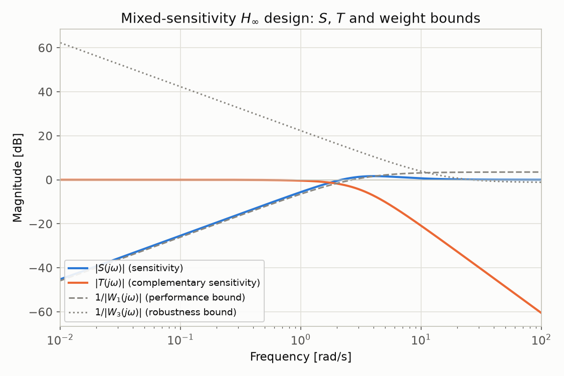
The peak sensitivity \(\max|S|=1.212\) is a good value (generally, below 2 is the rule of thumb). The core small-gain quantity \(\max|W_3T|=0.139<1\) holds, which theoretically guarantees that the closed loop remains stable no matter which uncertainty is realized, as long as it stays within the normalized bound \(\|\Delta\|_\infty\leq1\) assumed for the actuator-lag uncertainty (this is the same \(M=W_3T\) used in the small-gain numerical check earlier).
The figure below overlays the sensitivity function \(S\) and complementary sensitivity function \(T\) with their respective design bounds \(1/W_1\) (performance bound) and \(1/W_3\) (robustness bound). \(S\) staying below \(1/W_1\) at low frequency (good tracking performance) and \(T\) staying below \(1/W_3\) at high frequency (robustness) visualize the fundamental performance/robustness trade-off.
Comparison with a PID Controller
For comparison, we prepared a PID controller tuned using the ITAE-optimal criterion for a third-order system. Matching the closed-loop characteristic polynomial to \(s^3+1.75\omega_ns^2+2.15\omega_n^2s+\omega_n^3\) (with \(\omega_n=3\,\mathrm{rad/s}\) ) gives
\[ K_d = 1.75\omega_n - c = 4.850,\quad K_p = 2.15\omega_n^2-k_{\mathrm{nom}}=15.350,\quad K_i=\omega_n^3=27.000 \]wn_c = 3.0
Kd = 1.75*wn_c - c
Kp = 2.15*wn_c**2 - k_nom
Ki = wn_c**3
PID = ct.tf([Kd, Kp, Ki], [1, 0])
print(f"PID gains: Kp={Kp:.3f} Ki={Ki:.3f} Kd={Kd:.3f}")
PID gains: Kp=15.350 Ki=27.000 Kd=4.850
We compared step responses for these two controllers across four scenarios.
| Scenario | Controller | Overshoot | 2% settling time | Closed-loop max \(\mathrm{Re}(\text{pole})\) |
|---|---|---|---|---|
| Nominal (\(k=4.0\) , no lag) | H∞ | 0.90% | 1.300 s | −0.2000 |
| Nominal | PID | 17.08% | 1.984 s | −1.5629 |
| Design-model uncertainty (\(k=4.0\) + lag) | H∞ | 4.03% | 2.040 s | −0.2000 |
| Design-model uncertainty | PID | 31.98% | 2.322 s | −1.7792 |
| Stress test (\(k=3.2\) + lag) | H∞ | 20.74% | 97.19 s | −0.0230 |
| Stress test (\(k=3.2\) + lag) | PID | 35.33% | 2.454 s | −1.6922 |
| Stress test (\(k=4.8\) + lag) | H∞ | 8.15% | 6.369 s | −0.4106 |
| Stress test (\(k=4.8\) + lag) | PID | 28.83% | 2.178 s | −1.8475 |
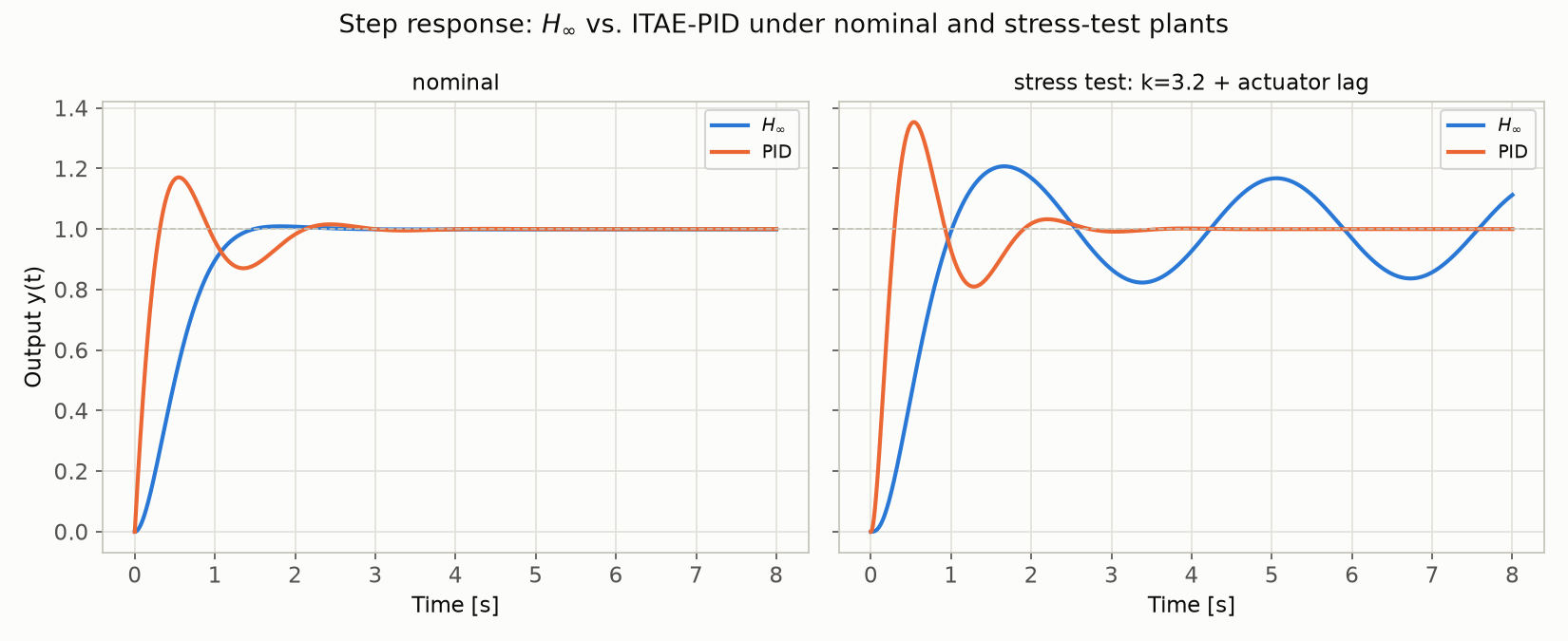
Within the “design-model uncertainty” (only the actuator lag explicitly accounted for in \(W_3\) ), H-infinity control’s overshoot of 4.03% is far below PID’s 31.98%, showing the benefit of robustness exactly as guaranteed by the small gain theorem. The figure below (left: nominal, right: stress test) shows this contrast visually.
Caveat: The Small-Gain Guarantee Only Covers the Assumed Uncertainty Class
However, an interesting reversal occurred in the “stress test” (adding a variation in the spring constant \(k\) , which was never included in the \(W_3\) design, on top of the actuator lag). For \(k=3.2\) (20% below nominal), the real part of the H-infinity closed loop’s dominant pole shrinks to just \(-0.023\) , right next to the imaginary axis, and the 2% settling time balloons to 97.19 seconds (about 75 times the 1.30 seconds seen at nominal). By contrast, PID control converges in 2.45 seconds in this same scenario — its overshoot is larger, but in practice it behaved far more robustly.
Pushing \(k\) lower still, bisection shows that the H-infinity controller actually goes unstable around \(k\approx3.086\) (about 22.9% below nominal, combined with the actuator lag).
lo, hi = 2.8, 4.0
for _ in range(40):
    mid = (lo + hi) / 2
    G_true = plant(mid, lag=True)
    stable = np.all(ct.poles(ct.feedback(G_true*K, 1)).real < 0)
    if stable:
        hi = mid
    else:
        lo = mid
print(f"H-infinity controller unstable below k = {hi:.4f}")
H-infinity controller unstable below k = 3.0858
This is by no means a sign that H-infinity control is inferior — it demonstrates a critically important limitation: the robust-stability guarantee from the small gain theorem and the Bounded Real Lemma only extends to the structure and size of the uncertainty \(\Delta\) that was modeled at design time. Our \(W_3\) represented only one specific kind of uncertainty (actuator lag); a different kind of (structured, parametric) uncertainty — the spring constant — was never accounted for at all. The comfortable margin \(\max|W_3T|=0.139\) is meaningful only with respect to “uncertainty in the actuator-lag direction,” and offers no guarantee whatsoever against perturbations in other directions.
Handling multiple, structured sources of uncertainty simultaneously properly requires structured singular value \(\mu\) (mu) analysis and D-K iteration — normalizing each uncertainty block individually in a multi-input multi-output uncertainty structure (Doyle, 1982; Skogestad & Postlethwaite, Multivariable Feedback Control, 2005, Ch. 8). That is beyond the scope of this article, but the lesson — “H-infinity control is not universally robust; it only carries a mathematically proven guarantee against the uncertainty explicitly modeled at design time” — is an essential caveat when modeling uncertainty in practice.
Disturbance Rejection Performance
Finally, we compare the output-disturbance rejection performance for the nominal plant.
Sdist_hinf = ct.feedback(1, G_nom*K)
Sdist_pid = ct.feedback(1, G_nom*PID)
Both controllers include integral action, so steady-state error converges to zero in both cases; the transient convergence speed followed the same trend as the step response (H∞: 1.30 s, PID: 1.98 s, for the nominal plant).
Summary
- The H-infinity norm \(\|T_{zw}\|_\infty=\sup_\omega\bar\sigma(T_{zw}(j\omega))\)
is the induced norm for finite-energy (\(L_2\)
) inputs, representing the worst-case gain. A numerical experiment confirmed that
control.linfnormand a brute-force search agree to 6 decimal places. - The small gain theorem — \(\|M\|_\infty\|\Delta\|_\infty<1\) — is a sufficient condition provable two ways: convergence of a Neumann series (operator theory) and continuous deformation of the Nyquist stability criterion (complex analysis). The numerical experiment showed the theoretical stability limit (\(1/\|M\|_\infty=7.179\) ) matched the actual instability point (\(\delta\approx7.255\) ) within about 1% conservatism.
- The standard H-infinity control problem is formulated as the lower linear fractional transformation of a generalized plant \(P\) , \(F_l(P,K)=P_{11}+P_{12}K(I-P_{22}K)^{-1}P_{21}\) , and the mixed-sensitivity problem can be written down explicitly as a special case.
- The H-infinity algebraic Riccati equation can be derived from the saddle-point condition (the HJI equation) of the state-feedback problem via completing the square, and the corresponding Hamiltonian matrix having no eigenvalues on the imaginary axis is the existence condition for a solution (the test used in gamma iteration). The numerical example confirmed that the existence of a solution and closed-loop stability both vanish simultaneously at the boundary \(\gamma_{\min}\approx1.599\) .
- The Bounded Real Lemma applies this idea to a fixed system with no controller, and we numerically verified that \(\|G\|_\infty<\gamma\)
and Riccati-equation solvability are equivalent, matching two independent algorithms (Hamiltonian eigenvalue testing and
linfnorm) to 12 decimal places. - In the numerical example, an H-infinity controller designed with
control.mixsyn(\(\gamma=1.149\) ) for a mass-spring-damper system with actuator-lag uncertainty was substantially more robust than PID within the assumed uncertainty class (4.03% vs. 31.98% overshoot), but the guarantee does not extend to an uncertainty type not modeled at design time (variation in the spring constant), and the closed loop goes unstable around \(k\approx3.086\) . This experiment demonstrated concretely that a robust-control guarantee is always contingent on what was actually modeled as uncertainty.
Related Articles
- Bode Plot: Reading and Creating Frequency Response Diagrams with Python Implementation - Covers the classical stability margins (gain margin, phase margin) with worked numerical examples. This article’s robust stability generalizes those classical indicators to explicitly modeled uncertainty.
- Reading Nyquist Plots, Root Locus, and Stability Margins with Python - Covers the Nyquist stability criterion \(Z=N+P\) used in the small gain theorem’s proof.
- Fundamentals of PID Control - The theoretical basis of the PID controller compared against H-infinity control in this article.
- PID Control in Python: Simulation and Tuning - A deeper dive into implementing and tuning PID controllers.
- Extended Kalman Filter (EKF): Theory and Python Implementation - A sister field whose references include the relationship between state estimation and H-infinity filtering.
References
- Doyle, J. C., Glover, K., Khargonekar, P. P., & Francis, B. A. (1989). “State-space solutions to standard H2 and H∞ control problems.” IEEE Transactions on Automatic Control, 34(8), 831–847.
- Zhou, K., Doyle, J. C., & Glover, K. (1996). Robust and Optimal Control. Prentice Hall.
- Skogestad, S., & Postlethwaite, I. (2005). Multivariable Feedback Control: Analysis and Design (2nd ed.). Wiley.
- Doyle, J. C. (1982). “Analysis of feedback systems with structured uncertainties.” IEE Proceedings D, 129(6), 242–250.
- python-control:
hinfsyndocumentation - SLICOT: Subroutine Library in Systems and Control Theory
Related Tools
- DevToolBox - Free Developer Tools - 90+ developer tools including JSON formatting and regex testing
- CalcBox - Everyday Calculation Tools - 60+ calculation tools including statistics and frequency conversion