In statistics, a moment is a quantitative measure that characterizes the shape of a probability distribution. The concept is borrowed from physics (where moment refers to rotational force) and applied to statistics. Moments are used to quantitatively describe the center, spread, asymmetry, and tail behavior of a random variable \(X\) ’s distribution.
This article works through the definitions of moments up to skewness and kurtosis, and then addresses a question textbooks often gloss over beyond the variance case: is a moment computed from a finite sample an unbiased estimator of the true population moment? We answer this both analytically and with an executed Monte Carlo study, extending the question to skewness and kurtosis as well.
Definition of Moments
Given a random variable \(X\) with probability density function (or probability mass function) \(f(x)\) , the \(n\) -th moment about the origin \(\mu'_n\) is defined as:
\[ \mu'_n = \mathbb{E}[X^n] = \int_{-\infty}^{\infty} x^n f(x) dx \]The \(n\) -th moment about the mean \(\mu = \mathbb{E}[X]\) (central moment) \(\mu_n\) is defined as:
\[ \mu*n = \mathbb{E}[(X - \mu)^n] = \int*{-\infty}^{\infty} (x - \mu)^n f(x) dx \]Because central moments are taken about the mean, they do not depend on the location of the distribution — only on its shape (scale, asymmetry, tail weight). Starting from the \(k\) -th central moment \(\mu_k\) , we go through the meaning of each order below.
Meaning of Lower-Order Moments
0th Moment
- 0th moment about the origin: \(\mu'_0 = \int_{-\infty}^{\infty} x^0 f(x) dx = \int_{-\infty}^{\infty} f(x) dx = 1\) This represents the fundamental property of probability that the integral of the probability density function over the entire domain equals 1.
1st Moment
- 1st moment about the origin: \(\mu'_1 = \int_{-\infty}^{\infty} x^1 f(x) dx = \mathbb{E}[X] = \mu\) This represents the mean (expected value) of the random variable. It indicates the center of the distribution.
2nd Moment
- 2nd central moment: \(\mu_2 = \mathbb{E}[(X - \mu)^2] = \sigma^2\) This represents the variance of the random variable. It indicates the spread of the distribution.
Meaning of Higher-Order Moments
3rd Moment (Skewness)
Normalizing the 3rd central moment \(\mu_3\) by the scale \(\sigma^3\) gives the skewness \(\gamma_1\) of a distribution:
\[ \gamma_1 = \frac{\mu_3}{\sigma^3} = \frac{\mathbb{E}[(X-\mu)^3]}{\left(\mathbb{E}[(X-\mu)^2]\right)^{3/2}} \]Dividing by \(\sigma^3\) makes \(\gamma_1\) dimensionless, so it compares shape alone, independent of the unit \(X\) is measured in. Skewness indicates the direction and magnitude of asymmetry:
- \(\gamma_1 > 0\) : The distribution is right-skewed (has a longer right tail) — large-value outliers are relatively more common
- \(\gamma_1 < 0\) : The distribution is left-skewed (has a longer left tail)
- \(\gamma_1 = 0\) : The distribution is symmetric (e.g., normal distribution — though the converse need not hold; a distribution can be asymmetric in ways the third moment doesn’t detect)
4th Moment (Kurtosis)
Similarly, normalizing the 4th central moment \(\mu_4\) by \(\sigma^4\) and subtracting 3 (the value for a normal distribution) gives the (excess) kurtosis \(\gamma_2\) :
\[ \gamma_2 = \frac{\mu_4}{\sigma^4} - 3 \]That the (non-excess) kurtosis of a normal distribution equals exactly 3 can be verified from the moments of the normal distribution (\(\mathbb{E}[Z^4]=3\) for \(Z \sim N(0,1)\) ). Subtracting 3 lets excess kurtosis directly measure the “deviation from normal”:
- \(\gamma_2 > 0\) : Heavier tails than a normal distribution (higher excess kurtosis)
- \(\gamma_2 < 0\) : Lighter tails than a normal distribution
- \(\gamma_2 = 0\) : Same tail weight as a normal distribution
A common misconception about kurtosis: Kurtosis is frequently described as measuring “peakedness” — how sharp the center of the distribution is. This is not quite right. Because \(\gamma_2\) is defined via the 4th moment \(\mathbb{E}[(X-\mu)^4]\) , and raising a deviation to the 4th power weights the tails (\(|X-\mu|\) large) far more heavily than the region near the center. Westfall (2014, The American Statistician, “Kurtosis as Peakedness, 1905–2014. R.I.P.”) makes exactly this point: kurtosis primarily measures tail heaviness (propensity for outliers), not the sharpness of the central peak. Distributions with high kurtosis, such as the Laplace or Student-\(t\) , do tend to have a sharp central peak, but that is a side effect of heavy tails, not a direct consequence — assuming “high kurtosis \(\Rightarrow\) sharp peak” in general is a mistake (a uniform distribution, for instance, is flat and tail-less yet has lower kurtosis than a normal distribution). We will keep using the word “kurtosis” below, but it should be understood as a measure of tail weight, not peakedness.
Moments are fundamental tools for capturing various characteristics of probability distributions and play an important role in understanding data properties in data analysis and machine learning. In practice, however, we never observe the true population \(\mu, \sigma^2, \gamma_1, \gamma_2\) directly — we can only estimate them from a finite sample. The rest of this article examines a property those estimators may or may not have: unbiasedness.
Sample Moments and Unbiasedness: The Case of Variance
Let \(X_1, \dots, X_n\) be i.i.d. draws from a distribution with mean \(\mu\) and variance \(\sigma^2\) , and let \(\bar X = \frac{1}{n}\sum_{i=1}^n X_i\) be the sample mean. The most naive estimator of the variance is
\[ \hat\sigma^2 = \frac{1}{n}\sum\_{i=1}^n (X_i - \bar X)^2 \]This looks like the natural plug-in estimator obtained by replacing \(\mu\) with \(\bar X\) and the expectation with a sample average in the definition \(\sigma^2 = \mathbb{E}[(X-\mu)^2]\) . It turns out, however, to be biased.
Why \(\hat\sigma^2\) Is Biased (Derivation)
The key is the following algebraic identity:
\[ \sum*{i=1}^n (X_i - \bar X)^2 = \sum*{i=1}^n (X_i - \mu)^2 - n(\bar X - \mu)^2 \tag{1}\]Derivation: Write \(X_i - \bar X = (X_i - \mu) - (\bar X - \mu)\) , square both sides, and sum:
\[ \sum_i (X_i-\bar X)^2 = \sum_i (X_i-\mu)^2 - 2(\bar X - \mu)\sum_i(X_i-\mu) + n(\bar X-\mu)^2 \]Since \(\sum_i (X_i - \mu) = n(\bar X - \mu)\) , the middle term becomes \(-2n(\bar X-\mu)^2\) , giving
\[ \sum_i (X_i-\bar X)^2 = \sum_i (X_i-\mu)^2 - 2n(\bar X-\mu)^2 + n(\bar X-\mu)^2 = \sum_i (X_i-\mu)^2 - n(\bar X-\mu)^2 \]which establishes (1). This identity says that the spread around the sample mean is always smaller than the spread around the true mean, by exactly the sampling error of \(\bar X\) itself — because \(\bar X\) is computed from the same data, it is inevitably “pulled toward” the data.
Taking expectations of both sides: \(\mathbb{E}[(X_i-\mu)^2]=\sigma^2\) , so the left sum’s expectation is \(n\sigma^2\) . Also \(\mathrm{Var}(\bar X) = \sigma^2/n\) , so \(\mathbb{E}[n(\bar X-\mu)^2] = n\cdot\sigma^2/n = \sigma^2\) . Hence
\[ \mathbb{E}\left[\sum_i (X_i-\bar X)^2\right] = n\sigma^2 - \sigma^2 = (n-1)\sigma^2 \]Dividing both sides by \(n\) :
\[ \mathbb{E}[\hat\sigma^2] = \frac{n-1}{n}\sigma^2 \tag{2}\]That is, \(\hat\sigma^2\) always underestimates the true variance (bias \(= -\sigma^2/n\) ). Crucially, this derivation makes no assumption about the shape of the population distribution (Gaussian or otherwise) — it follows purely from \(\mathrm{Var}(\bar X)=\sigma^2/n\) and linearity of expectation, a fully general result for any distribution with finite variance.
Bessel’s Correction: Dividing by \(n-1\) Makes It Exactly Unbiased
Equation (2) immediately suggests multiplying by \(n/(n-1)\) to fix the bias:
\[ s^2 = \frac{n}{n-1}\hat\sigma^2 = \frac{1}{n-1}\sum\_{i=1}^n (X_i-\bar X)^2 \tag{3}\] \[ \mathbb{E}[s^2] = \frac{n}{n-1}\cdot\frac{n-1}{n}\sigma^2 = \sigma^2 \]This is Bessel’s correction. Dividing by the degrees of freedom \(n-1\) (subtracting one for the degree of freedom “used up” estimating \(\bar X\) ) yields an estimator that is exactly unbiased for any distribution. This distribution-free exactness is the key contrast with skewness and kurtosis, examined next.
Why Unbiased Estimation of Skewness and Kurtosis Is Trickier
By the same logic as variance, one might hope to “correct” skewness and kurtosis the same way. Indeed, scipy.stats.skew / scipy.stats.kurtosis return the following adjusted Fisher–Pearson standardized moment coefficients when bias=False is passed:
where \(m_k = \frac{1}{n}\sum_i (X_i-\bar X)^k\) is the naive sample central moment. These correction factors trace back to Fisher (1930), and the name “\(G_1, G_2\) ” together with the label “bias-corrected” invites the assumption that they behave like \(s^2\) — exactly unbiased for any distribution. That assumption is wrong, for two compounding reasons.
(1) Ratios of unbiased estimators are not generally unbiased. For variance, \(\hat\sigma^2\) itself was the estimator being corrected. Skewness and kurtosis, by contrast, are defined as a ratio of an estimator of the 3rd (4th) central moment to a power of an estimator of the variance. Even if \(A\) and \(B\) are each unbiased (\(\mathbb{E}[A]=\alpha\) , \(\mathbb{E}[B]=\beta\) ), in general \(\mathbb{E}[A/B] \neq \alpha/\beta\) (the expectation of a ratio is not the ratio of expectations — related to Jensen’s inequality). No matter how carefully the numerator and denominator are made unbiased individually, the ratio itself is not guaranteed to be unbiased.
(2) The \(G_1, G_2\) correction factors are themselves derived under a normality assumption. Coefficients like \(\sqrt{n(n-1))}/(n-2)\) and \((n-1)/((n-2)(n-3))\) come from small-sample/asymptotic expansions that assume the population is approximately Gaussian. As Joanes & Gill (1998, The Statistician, “Comparing measures of sample skewness and kurtosis”) point out, these corrections are not generally unbiased for non-normal populations. \(G_1, G_2\) are estimators tuned to have smaller bias than \(g_1, g_2\) if the population happens to be normal — not estimators that are unbiased for any distribution.
This distinction matters: the \(n-1\) correction for variance is a distribution-free algebraic fact, while the skewness/kurtosis “corrections” are distribution-dependent approximations. Below we verify this claim directly with code.
Verification via Monte Carlo Simulation
We use three distributions, each with an analytically known set of true moments, and for each sample size \(n\) we generate a large number of simulated samples to measure the empirical bias (mean of the estimator across repetitions minus the true value) of each estimator.
| Distribution | Mean | Variance | Skewness \(\gamma_1\) | Excess kurtosis \(\gamma_2\) |
|---|---|---|---|---|
| Gaussian \(N(0,1)\) | 0 | 1 | 0 | 0 |
| Exponential(scale=1) | 1 | 1 | 2 | 6 |
| Student-\(t\) (df=5) | 0 | \(5/3\) | 0 | \(6\) (\(=6/(5-4)\) ) |
The Gaussian is the baseline case where the skewness/kurtosis corrections are theoretically designed to work well. The exponential is an asymmetric, heavy-tailed case with both nonzero skewness and kurtosis. Student-\(t\) (df=5) has zero skewness (symmetric) but the same excess kurtosis of 6 as the exponential — comparing the three lets us disentangle whether the correction failures are driven by asymmetry or purely by tail weight.
import numpy as np
from scipy import stats

rng = np.random.default_rng(20210527)
M = 20000  # Monte Carlo repetitions

dists = {
    "gaussian":    dict(sampler=lambda shape, rng: rng.standard_normal(shape),
                         var=1.0, skew=0.0, exkurt=0.0),
    "exponential": dict(sampler=lambda shape, rng: rng.exponential(1.0, size=shape),
                         var=1.0, skew=2.0, exkurt=6.0),
    "student_t5":  dict(sampler=lambda shape, rng: rng.standard_t(df=5, size=shape),
                         var=5/3, skew=0.0, exkurt=6.0),
}

def run_for_n(dist, n, M, rng):
    x = dist["sampler"]((M, n), rng)                    # shape (M, n)
    d = x - x.mean(axis=1, keepdims=True)
    var_naive  = np.mean(d**2, axis=1)                  # naive: 1/n
    var_bessel = np.sum(d**2, axis=1) / (n - 1)         # Bessel: 1/(n-1)
    skew_biased = stats.skew(x, axis=1, bias=True)       # g1
    skew_adj    = stats.skew(x, axis=1, bias=False)      # G1
    kurt_biased = stats.kurtosis(x, axis=1, bias=True)   # g2 (excess)
    kurt_adj    = stats.kurtosis(x, axis=1, bias=False)  # G2 (excess)
    return var_naive, var_bessel, skew_biased, skew_adj, kurt_biased, kurt_adj

n = 30
for name, dist in dists.items():
    vn, vb, sb, sa, kb, ka = run_for_n(dist, n, M, rng)
    print(name)
    print(f"  variance   naive  bias={vn.mean()-dist['var']:+.5f}  (theory -var/n={-dist['var']/n:+.5f})")
    print(f"  variance   Bessel bias={vb.mean()-dist['var']:+.5f}")
    print(f"  skewness   g1     bias={sb.mean()-dist['skew']:+.5f}")
    print(f"  skewness   G1     bias={sa.mean()-dist['skew']:+.5f}")
    print(f"  exkurt     g2     bias={kb.mean()-dist['exkurt']:+.5f}")
    print(f"  exkurt     G2     bias={ka.mean()-dist['exkurt']:+.5f}")
Running this with \(n=30\) , \(M=20{,}000\) repetitions gives the following (Monte Carlo standard errors are all in the 0.006–0.024 range, well below the biases reported, so these are statistically significant):
| Distribution | Estimator | True value | Mean estimate | Bias |
|---|---|---|---|---|
| Gaussian | Variance (naive, ÷n) | 1.0000 | 0.96758 | −0.03242 (theory −0.03333) |
| Gaussian | Variance (Bessel, ÷(n−1)) | 1.0000 | 1.00095 | +0.00095 |
| Gaussian | Skewness \(g_1\) (bias=True) | 0.0000 | 0.00300 | +0.00300 |
| Gaussian | Skewness \(G_1\) (bias=False) | 0.0000 | 0.00316 | +0.00316 |
| Gaussian | Excess kurtosis \(g_2\) (bias=True) | 0.0000 | −0.19018 | −0.19018 |
| Gaussian | Excess kurtosis \(G_2\) (bias=False) | 0.0000 | 0.00401 | +0.00401 |
| Exponential | Variance (naive) | 1.0000 | 0.96405 | −0.03595 |
| Exponential | Variance (Bessel) | 1.0000 | 0.99729 | −0.00271 |
| Exponential | Skewness \(g_1\) | 2.0000 | 1.47841 | −0.52159 |
| Exponential | Skewness \(G_1\) | 2.0000 | 1.55738 | −0.44262 |
| Exponential | Excess kurtosis \(g_2\) | 6.0000 | 2.23436 | −3.76564 |
| Exponential | Excess kurtosis \(G_2\) | 6.0000 | 2.88715 | −3.11285 |
| Student-\(t\) (5) | Variance (naive) | 1.6667 | 1.60942 | −0.05724 |
| Student-\(t\) (5) | Variance (Bessel) | 1.6667 | 1.66492 | −0.00175 |
| Student-\(t\) (5) | Skewness \(g_1\) | 0.0000 | −0.00869 | −0.00869 |
| Student-\(t\) (5) | Skewness \(G_1\) | 0.0000 | −0.00915 | −0.00915 |
| Student-\(t\) (5) | Excess kurtosis \(g_2\) | 6.0000 | 1.07706 | −4.92294 |
| Student-\(t\) (5) | Excess kurtosis \(G_2\) | 6.0000 | 1.51094 | −4.48906 |
These results clearly confirm the previous section’s predictions.
- Variance: The naive estimator is biased negatively by the theoretical \(-\sigma^2/n\) amount in all three distributions, and after Bessel’s correction the bias is within \(\pm0.003\) (Monte Carlo noise) for all three. This numerically confirms the claim that the correction is exactly unbiased regardless of distribution.
- Skewness: For the Gaussian (true skewness 0), both \(g_1\) and \(G_1\) have essentially zero bias — there’s nothing for the correction to fix when the true value is already 0. For the exponential (true skewness 2), \(g_1\) ’s bias of \(-0.522\) improves only to \(-0.443\) with \(G_1\) — still over 20% of the true value. For the symmetric Student-\(t\) (5) (true skewness 0), both estimators are again nearly unbiased, showing that the leading-order skewness bias scales with the population skewness itself — for symmetric distributions there’s essentially no skewness bias to begin with, regardless of kurtosis.
- Kurtosis: For the Gaussian, \(g_2\) ’s bias of \(-0.190\) is corrected to \(+0.004\) by \(G_2\) — nearly perfect, exactly as designed for a normal population. But for the exponential and Student-\(t\) (5) (both with true excess kurtosis 6), even after \(G_2\) correction the biases remain enormous at \(-3.11\) and \(-4.49\) respectively. The \(G_2\) correction is barely useful in either the asymmetric (exponential) or symmetric-but-heavy-tailed (Student-\(t\) ) case.
These experiments confirm Joanes & Gill’s (1998) claim in concrete numbers: the bias=False corrections for skewness/kurtosis are normality-based approximations, not estimators that are unbiased in general.
Bias vs. Sample Size \(n\)
The table above is a single snapshot at \(n=30\) . The figures below track the same empirical bias, again with \(M=20{,}000\) repetitions per point, as \(n\) ranges from 5 to 2000.
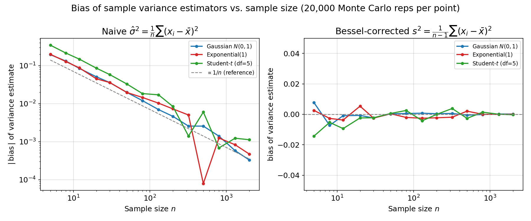
The naive variance estimator’s bias tracks the \(\propto 1/n\) reference line closely for all three distributions, consistent with equation (2). After Bessel’s correction, the bias is near zero even at the extreme case of \(n=5\) , confirming unbiasedness for any \(n\) , any distribution.
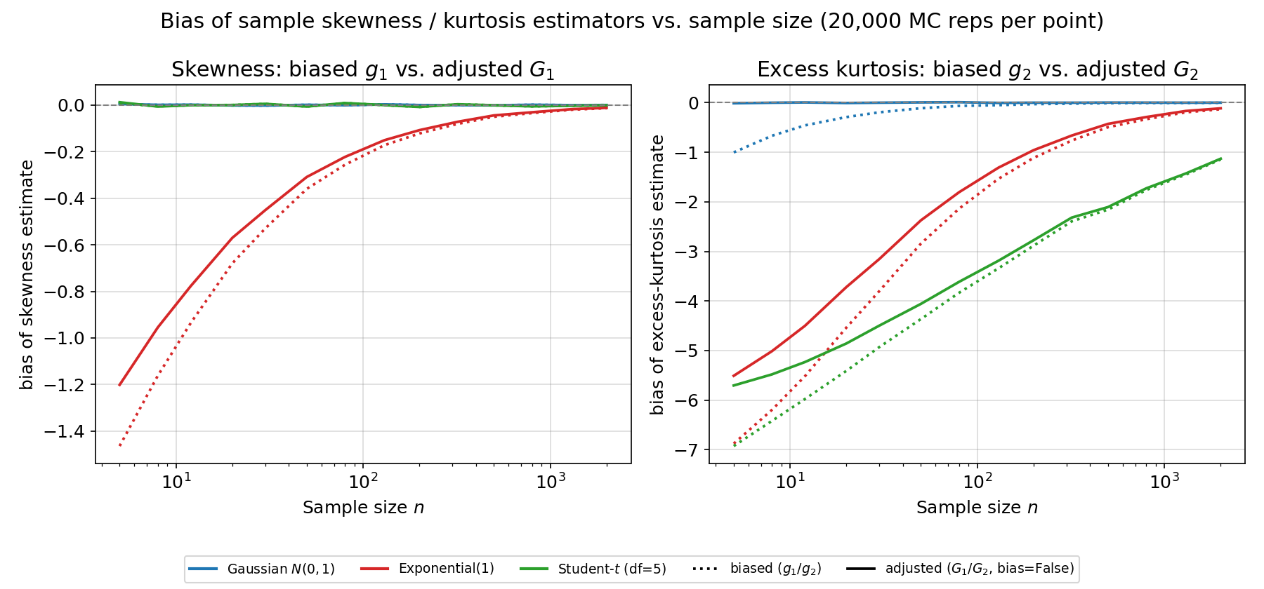
In both panels, the Gaussian (blue) hovers near zero regardless of correction. For the exponential (red) and Student-\(t\) (5) (green), the bias=False correction (solid) reduces the bias somewhat compared to bias=True (dotted), but a non-negligible bias remains even at several hundred samples — visually confirming that the “correction” is only an approximate mitigation in finite samples, not a fix.
One further caveat applies to the Student-\(t\) (5) kurtosis estimator specifically. The \(k\) -th moment of a \(t\) distribution with \(\nu\) degrees of freedom is finite only for \(k < \nu\) . With \(\mathrm{df}=5\) , the 4th moment is just barely finite (\(4<5\) ), but the asymptotic variance of the kurtosis estimator itself requires the 8th moment to be finite, and \(8 \not< 5\) means it is infinite. Measuring the standard deviation of \(\hat g_2\) as \(n\) grows,
for n in [200, 500, 2000, 8000]:
    x = rng.standard_t(df=5, size=(20000, n))
    k = stats.kurtosis(x, axis=1, bias=True)
    print(n, k.std(), k.std() * np.sqrt(n))
gives std * sqrt(n) values of roughly 71 at \(n=200\)
and roughly 1589 at \(n=8000\)
— increasing with \(n\)
(for an estimator obeying a standard central limit theorem, std * sqrt(n) should stay roughly constant). This means that for heavy-tailed distributions like Student-\(t\)
(5), the kurtosis estimator itself converges far slower than the usual \(1/\sqrt{n}\)
rate, and estimating its bias reliably requires many more repetitions than usual. Estimating higher-order moments for heavy-tailed distributions is a case where not just the bias, but the very question of whether the estimate is stable at all, needs care.
Practical Relevance
Bias in skewness/kurtosis estimation is especially relevant wherever heavy-tailed distributions show up, such as financial volatility analysis. This blog’s
GARCH(1,1) in Python
models the conditional variance of stock returns with GARCH(1,1); it’s well known that return distributions themselves tend to be heavier-tailed than normal (positive excess kurtosis). If you estimate kurtosis on a window of a few hundred to a few thousand observations for a risk metric, this article’s findings are a reminder that even the bias=False “correction” can leave a substantial residual bias the further the true distribution is from Gaussian.
Summary
- From the \(k\) -th central moment \(\mu_k=\mathbb{E}[(X-\mu)^k]\) , skewness \(\gamma_1=\mu_3/\sigma^3\) (asymmetry) and excess kurtosis \(\gamma_2=\mu_4/\sigma^4-3\) (tail weight — not peakedness) are defined.
- The naive sample variance estimator \(\hat\sigma^2=\frac{1}{n}\sum(X_i-\bar X)^2\) satisfies \(\mathbb{E}[\hat\sigma^2]=\frac{n-1}{n}\sigma^2\) , underestimating the true variance exactly, for any distribution. Bessel’s correction \(s^2=\frac{1}{n-1}\sum(X_i-\bar X)^2\) is exactly unbiased, for any distribution.
- The
bias=Falseskewness/kurtosis corrections (\(G_1, G_2\) ) are, for two reasons — ratios of unbiased estimators need not be unbiased, and the correction factors themselves assume normality — not generally unbiased for non-normal distributions. Our Monte Carlo study confirmed that the kurtosis correction works almost perfectly for the Gaussian, but leaves substantial bias at several hundred samples for the exponential and Student-\(t\) (5). - For distributions with extremely heavy tails (e.g. low-df \(t\) distributions), the higher-moment estimators themselves converge slowly, requiring far more repetitions to even measure their bias reliably.