This article shows how to visualize 3D data and save it as an animated GIF using Matplotlib and NumPy. This technique is especially useful for representing 3D data that changes over time.
Generated GIF
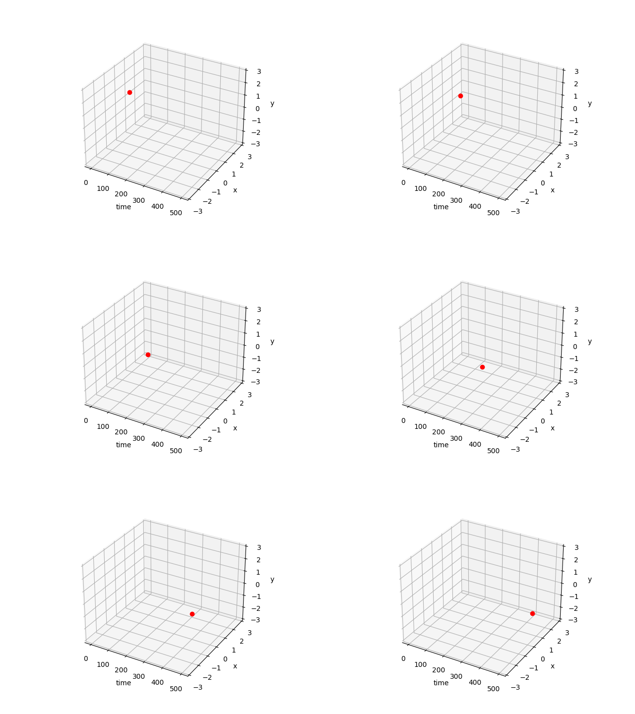
Code
import numpy as np
import matplotlib.pyplot as plt
import matplotlib.animation as animation
from mpl_toolkits.mplot3d import Axes3D # Required for 3D plotting

def make_animation(data_frames, filename="animation.gif"):
    """
    Create and save a 3D data animation as a GIF.

    :param data_frames: List of 3D coordinates (X, Y, Z) for each frame.
                        Example: [[X_frame1, Y_frame1, Z_frame1], [X_frame2, Y_frame2, Z_frame2], ...]
    :param filename: Path to save the GIF file.
    """
    print("Generating frames...")

    fig = plt.figure(figsize=(8, 6)) # Specify figure size
    ax = fig.add_subplot(111, projection='3d')

    # Set axis labels
    ax.set_xlabel('X-axis')
    ax.set_ylabel('Y-axis')
    ax.set_zlabel('Z-axis')

    # Auto-adjust axis range to fit data, or set manually
    # ax.set_xlim(-500, 500) # Example
    # ax.set_ylim(-3, 3)
    # ax.set_zlim(-3, 3)

    ims = [] # List to store Artist objects for each frame

    for i, (X, Y, Z) in enumerate(data_frames):
        # Display progress
        progress = (i + 1) * 100 / len(data_frames)
        print(f"\rProgress: {progress:.1f}%", end="")

        # 3D plot. marker='o' displays points, linestyle='None' hides lines
        im, = ax.plot(X, Y, Z, marker="o", color="red", linestyle='None') # Unpack with comma

        ims.append([im]) # ArtistAnimation expects a list of lists

    print("\nGenerating animation...")

    # Create animation
    # fig: The Figure object for the animation
    # ims: List of Artist objects for each frame
    # interval: Delay between frames (milliseconds)
    # blit: If True, only redraw changed parts for speed (may cause issues with complex 3D plots)
    ani = animation.ArtistAnimation(fig, ims, interval=50, blit=False)

    # Save animation
    # writer: Writer for saving the animation. May require 'ffmpeg' or 'imagemagick'.
    # fps: Frames per second
    ani.save(filename, writer='pillow', fps=20) # 'pillow' can save GIFs without external tools

    print(f"Animation saved to {filename}.")
    plt.show() # Display the animation

def main():
    # Generate sample data
    # 3D trajectory where sin and cos waves change with time t
    t = np.linspace(0, 20 * np.pi, 500) # 500 points from 0 to 20pi

    data_frames = []
    for i in range(len(t)):
        # Example: plot one point per frame
        X_val = t[i] / (20 * np.pi) * 5 # X-axis changes with time
        Y_val = np.sin(t[i])
        Z_val = np.cos(t[i])
        data_frames.append([[X_val], [Y_val], [Z_val]]) # Wrap each value in a list

    make_animation(data_frames, filename="sin_cos_3d_animation.gif")

if __name__ == '__main__':
  main()
Code Explanation
matplotlib.animation.ArtistAnimation: Creates an animation by passing a list of Artist objects returned by theplotfunction, which are drawn for each frame.fig.add_subplot(111, projection='3d'): Required for creating 3D plots.ax.plot(X, Y, Z, ...): Plots data in 3D space. Customize the appearance withmarker,color,linestyle, etc.ani.save(filename, writer='pillow', fps=20): Saves the animation as a GIF file.writer='pillow': Uses the Pillow library to generate the GIF. Requirespip install pillowbut does not need external tools likeffmpeg.fps: Frames Per Second, controls the animation speed.
- Progress bar: Uses
\rto overwrite the same line, displaying a progress indicator in the console.
Feel free to use this code as a reference to animate and visualize various 3D datasets.
Note that the code above uses ArtistAnimation (pre-build every frame’s Artists up front and pass them as a list). In the rest of this article we’ll use the more flexible FuncAnimation (a function called once per frame that mutates Artist properties in place) to dig into how animation actually works and where the common pitfalls are.
How FuncAnimation Actually Works: The Artist-Update Model and Blitting
Updating Artists in Place, Not Recreating Them
matplotlib.animation.FuncAnimation does not rebuild the whole figure every frame. Instead, it mutates the data of existing Artist objects (Line2D/Line3D, etc.). A typical implementation looks like this:
import numpy as np
import matplotlib.pyplot as plt
import matplotlib.animation as animation

t = np.linspace(0, 8 * np.pi, 150)
x = t / (8 * np.pi) * 5
y = np.sin(t)
z = np.cos(t)

fig = plt.figure(figsize=(6, 4.5))
ax = fig.add_subplot(111, projection="3d")
ax.set_xlim(0, 5)
ax.set_ylim(-1.2, 1.2)
ax.set_zlim(-1.2, 1.2)

(trail,) = ax.plot([], [], [], color="tab:red", lw=1.5)
(head,) = ax.plot([], [], [], color="tab:red", marker="o", linestyle="None")


def update(i):
    # Only mutate the properties of Artists that actually changed
    trail.set_data(x[: i + 1], y[: i + 1])
    trail.set_3d_properties(z[: i + 1])
    head.set_data([x[i]], [y[i]])
    head.set_3d_properties([z[i]])
    # With blit=True, only the Artists returned here are redrawn
    return trail, head


ani = animation.FuncAnimation(fig, update, frames=len(t), interval=40, blit=False)
ani.save("funcanimation_demo.gif", writer="pillow", fps=20)
The key idea is that update(i) replaces only the coordinates of existing Artists via set_data() / set_3d_properties(), and returns the tuple of updated Artists. Because it doesn’t need to pre-generate and hold every frame’s Artists in memory the way ArtistAnimation does, it’s more memory-efficient for long animations and is the more commonly used API.
What Blitting Actually Optimizes
With blit=True, Matplotlib redraws only the bounding-box region of Artists that changed, and reuses the pixels it previously cached via canvas.copy_from_bbox() for everything else (axis labels, gridlines, background, etc.). In other words, blitting optimizes away a full canvas re-rasterization, speeding up interactive on-screen display by skipping redraw work for unchanged regions.
However, there’s an important and easily overlooked fact here. When you call ani.save() to write a file, Matplotlib always draws every frame with blit=False internally, regardless of the blit value you passed. You can verify this directly in the Matplotlib 3.10.x/3.11.x source (Animation.save() in matplotlib/animation.py):
# matplotlib/animation.py (excerpt from Animation.save)
for data in zip(*[a.new_saved_frame_seq() for a in all_anim]):
    for anim, d in zip(all_anim, data):
        # TODO: See if turning off blit is really necessary
        anim._draw_next_frame(d, blit=False)
    writer.grab_frame(**savefig_kwargs)
The comment “TODO: See if turning off blit is really necessary” confirms this is deliberate. The reason is straightforward: writing to a file requires handing the encoder a complete bitmap for every single frame, and blitting’s core assumption — “redraw only the diff and reuse the cached canvas” — doesn’t apply to a save pipeline that isn’t displaying a persistent canvas on screen.
To verify this empirically, we saved a 3D animation that rotates its viewpoint every frame as a GIF with both blit=True and blit=False, then compared the output frames pixel by pixel.
import numpy as np
import matplotlib.pyplot as plt
import matplotlib.animation as animation
from PIL import Image, ImageSequence


def make_gif(blit, filename):
    fig = plt.figure(figsize=(4, 4))
    ax = fig.add_subplot(111, projection="3d")
    (line,) = ax.plot([0], [0], [0], marker="o", color="red")

    def update(i):
        line.set_data([np.cos(i / 5)], [np.sin(i / 5)])
        line.set_3d_properties([0])
        ax.view_init(elev=20, azim=i * 10)  # rotate the view every frame
        return (line,)

    ani = animation.FuncAnimation(fig, update, frames=6, blit=blit, interval=200)
    ani.save(filename, writer="pillow", fps=2)
    plt.close(fig)


make_gif(True, "blit_true.gif")
make_gif(False, "blit_false.gif")


def frames_of(path):
    im = Image.open(path)
    return [np.array(f.convert("RGB")) for f in ImageSequence.Iterator(im)]


f_true = frames_of("blit_true.gif")
f_false = frames_of("blit_false.gif")
identical = all(np.array_equal(a, b) for a, b in zip(f_true, f_false))
print(f"All {len(f_true)} frames identical between blit=True and blit=False saves: {identical}")
Output:
All 6 frames identical between blit=True and blit=False saves: True
As expected, the saved GIFs were pixel-for-pixel identical regardless of the blit value. In short, the blit parameter has zero effect when writing to GIF/MP4. Blitting only matters for interactive on-screen display via plt.show() (or a Jupyter widget).
Why Blitting Doesn’t Play Nicely with 3D Axes
Even restricted to interactive display, the combination of 3D Axes (Axes3D) and blitting has a well-known limitation. Matplotlib’s issue tracker has multiple reports that enabling blit=True for a 3D animation breaks mouse-driven rotation and zoom of the view (
matplotlib/matplotlib#8162
).
The technical reason: blitting composites the screen from “cached background pixels + the diff of changed Artists.” But in a 3D view, changing the camera (elev/azim/roll) requires recomputing the projection and depth ordering (Z-order) of the entire scene. That’s fundamentally different from the 2D case where “only this one Artist’s coordinates changed” — the cached background (panes and gridlines from before the rotation) becomes stale the instant the viewpoint changes. For that reason, interactively rotating a blitted 3D Axes is not officially recommended (use blit=False, or lean on the newer Matplotlib performance improvements discussed later in this article).
That said, as established above, for a workflow like this article’s — saving to GIF/MP4 — the value of blit is effectively moot, since saving always performs a full (blit=False-equivalent) redraw regardless. blit=True only matters when you want fast, real-time interactive display of 2D Axes via plt.show().
Writer/Backend Tradeoffs: PillowWriter (GIF) vs. FFMpegWriter (MP4)
The original code saves the animation as a GIF via writer='pillow', but Matplotlib can also save to MP4 (H.264) via FFMpegWriter. The two have the following tradeoffs:
| PillowWriter (GIF) | FFMpegWriter (MP4) | |
|---|---|---|
| External tooling | None (pip install pillow only) | Requires the ffmpeg binary |
| Color depth | 256-color palette (prone to banding) | Full color |
| Autoplay in a browser | Autoplays/loops directly via <img> | Requires a <video> element |
| File size / encode speed | Worse, as measured below | Better, as measured below |
The test machine had no system-wide ffmpeg installed (which ffmpeg found nothing), so we installed pip install imageio-ffmpeg, which bundles a static ffmpeg build, and pointed matplotlib.rcParams["animation.ffmpeg_path"] at it. Below is the code we actually ran, and the measured results.
import os
import time
import numpy as np
import matplotlib
import matplotlib.pyplot as plt
import matplotlib.animation as animation

# No system ffmpeg is available, so point Matplotlib at the imageio-ffmpeg binary
import imageio_ffmpeg

matplotlib.rcParams["animation.ffmpeg_path"] = imageio_ffmpeg.get_ffmpeg_exe()


def build_animation(n_frames, dpi):
    t = np.linspace(0, 8 * np.pi, n_frames)
    x, y, z = t / (8 * np.pi) * 5, np.sin(t), np.cos(t)

    fig = plt.figure(figsize=(6, 4.5), dpi=dpi)
    ax = fig.add_subplot(111, projection="3d")
    ax.set_xlim(0, 5)
    ax.set_ylim(-1.2, 1.2)
    ax.set_zlim(-1.2, 1.2)
    (trail,) = ax.plot([], [], [], color="tab:red", lw=1.5)
    (head,) = ax.plot([], [], [], color="tab:red", marker="o", linestyle="None")

    def update(i):
        trail.set_data(x[: i + 1], y[: i + 1])
        trail.set_3d_properties(z[: i + 1])
        head.set_data([x[i]], [y[i]])
        head.set_3d_properties([z[i]])
        return trail, head

    return fig, animation.FuncAnimation(fig, update, frames=n_frames, interval=40)


for n_frames in (60, 150, 300):
    fig, ani = build_animation(n_frames, dpi=100)
    t0 = time.perf_counter()
    ani.save(f"gif_{n_frames}.gif", writer="pillow", fps=20)
    gif_time = time.perf_counter() - t0
    gif_size = os.path.getsize(f"gif_{n_frames}.gif") / 1024
    plt.close(fig)

    fig, ani = build_animation(n_frames, dpi=100)
    t0 = time.perf_counter()
    ani.save(f"mp4_{n_frames}.mp4", writer=animation.FFMpegWriter(fps=20, codec="libx264"))
    mp4_time = time.perf_counter() - t0
    mp4_size = os.path.getsize(f"mp4_{n_frames}.mp4") / 1024
    plt.close(fig)

    print(
        f"frames={n_frames:4d}  GIF: {gif_size:8.1f} KB / {gif_time:5.2f} s   "
        f"MP4: {mp4_size:8.1f} KB / {mp4_time:5.2f} s   "
        f"size ratio(GIF/MP4)={gif_size / mp4_size:5.1f}x"
    )
Measured results (Apple Silicon Mac, Matplotlib 3.11.1, DPI=100 fixed):
frames=  60  GIF:    358.1 KB /  1.64 s   MP4:     31.5 KB /  0.72 s   size ratio(GIF/MP4)= 11.4x
frames= 150  GIF:    637.5 KB /  4.03 s   MP4:     41.3 KB /  1.77 s   size ratio(GIF/MP4)= 15.4x
frames= 300  GIF:   1088.7 KB /  7.97 s   MP4:     74.4 KB /  3.61 s   size ratio(GIF/MP4)= 14.6x
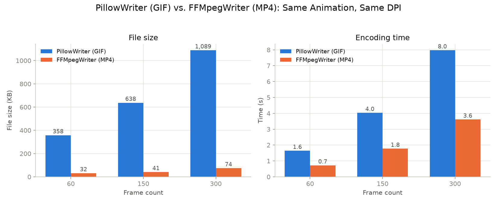
For the same animation at the same DPI, MP4 came out 11-15x smaller than GIF, and encoded roughly 2x faster. This is because GIF is quantized down to a 256-color palette, while H.264 performs genuine video compression using motion compensation and inter-frame prediction. For quick embedding via an <img> tag with autoplay — like this blog post — GIF’s simplicity still wins. But for animations with many frames or high resolution, it’s worth setting up ffmpeg and writing to MP4 instead.
Memory for Long Animations: Pre-Accumulating All Frames vs. Generating On-the-Fly
The original code accumulates every frame’s Artists into a list (ims) up front because ArtistAnimation requires it. It’s also common to see the underlying data (coordinate arrays) accumulated into a list before the animation loop even starts — but that approach uses memory proportional to the frame count.
FuncAnimation’s update() function, by contrast, can compute only the data needed for the current frame and discard it immediately afterward, which is clearly more memory-efficient for long, high-frame-count animations. We measured peak memory with tracemalloc to confirm this directly.
import gc
import tracemalloc
import numpy as np

N_POINTS = 200  # points per frame


def peak_mb_accumulate_all(n_frames, seed=123):
    """Bad: accumulate every frame's data into a list before animating"""
    tracemalloc.start()
    rng = np.random.default_rng(seed)
    frames = []
    for _ in range(n_frames):
        X = rng.normal(size=N_POINTS)
        Y = rng.normal(size=N_POINTS)
        Z = rng.normal(size=N_POINTS)
        frames.append((X, Y, Z))  # every frame stays resident here
    _, peak = tracemalloc.get_traced_memory()
    tracemalloc.stop()
    del frames
    gc.collect()
    return peak / 1e6


def peak_mb_on_the_fly(n_frames, seed=123):
    """Good: generate each frame inside the update function and discard it"""
    tracemalloc.start()
    rng = np.random.default_rng(seed)
    peak_seen = 0
    for _ in range(n_frames):
        X = rng.normal(size=N_POINTS)
        Y = rng.normal(size=N_POINTS)
        Z = rng.normal(size=N_POINTS)
        _, peak = tracemalloc.get_traced_memory()
        peak_seen = max(peak_seen, peak)
        # X, Y, Z go out of scope and are discarded here
    tracemalloc.stop()
    return peak_seen / 1e6


for n_frames in (500, 1000, 2000, 4000, 8000, 16000):
    list_mb = peak_mb_accumulate_all(n_frames)
    fly_mb = peak_mb_on_the_fly(n_frames)
    print(
        f"n_frames={n_frames:6d}  "
        f"pre-accumulated: {list_mb:8.3f} MB  "
        f"on-the-fly: {fly_mb:8.4f} MB  "
        f"ratio: {list_mb / fly_mb:8.1f}x"
    )
Output:
n_frames=   500  pre-accumulated:    3.476 MB  on-the-fly:   0.0088 MB  ratio:    395.3x
n_frames=  1000  pre-accumulated:    5.218 MB  on-the-fly:   0.0087 MB  ratio:    596.7x
n_frames=  2000  pre-accumulated:   10.433 MB  on-the-fly:   0.0087 MB  ratio:   1193.2x
n_frames=  4000  pre-accumulated:   20.866 MB  on-the-fly:   0.0087 MB  ratio:   2386.3x
n_frames=  8000  pre-accumulated:   41.732 MB  on-the-fly:   0.0087 MB  ratio:   4772.6x
n_frames= 16000  pre-accumulated:   83.465 MB  on-the-fly:   0.0087 MB  ratio:   9545.4x
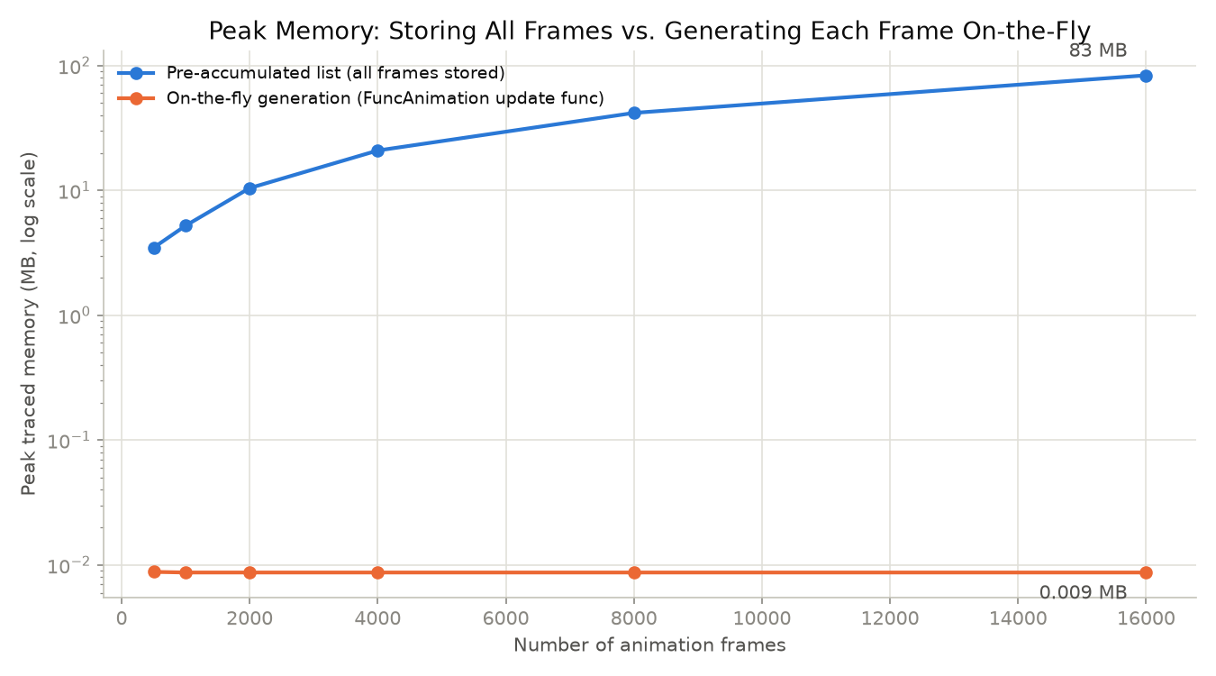
Pre-accumulating into a list grows memory linearly with frame count (each frame’s point cloud is roughly 200 points x 3 axes x 8 bytes ≈ 4.7 KB), reaching about 83 MB at 16,000 frames. Generating on-the-fly, by contrast, only ever holds “the current frame” in memory, staying at roughly 9 KB regardless of frame count. The difference is negligible for a few hundred frames, but for animations spanning tens of thousands of frames or high-resolution data, it can be the difference between a script that runs fine and one that runs out of memory. Prefer computing frame data inside update() whenever the source data allows it.
A Common Gotcha: Forgetting to Keep a Reference to the FuncAnimation Object
FuncAnimation / ArtistAnimation are ordinary Python objects, so like anything else they become eligible for garbage collection once nothing references them anymore. If you build ani = animation.FuncAnimation(...) inside a function and never return ani (i.e., the caller never assigns it to a variable), the object can be destroyed — and the animation can stop mid-run — even while it’s still supposed to be running. This bites people especially often inside a Jupyter Notebook cell wrapped in a function, or when an animation is created transiently inside a GUI callback.
import gc
import weakref
import matplotlib.pyplot as plt
import matplotlib.animation as animation


def make_animation_without_keeping_reference():
    fig, ax = plt.subplots()
    (line,) = ax.plot([], [])

    def update(i):
        line.set_data([0, 1], [0, i])
        return (line,)

    ani = animation.FuncAnimation(fig, update, frames=20, interval=10)
    # Return only a weakref, not ani itself
    # -> once this function returns, nothing holds a strong reference to ani
    return weakref.ref(ani), fig


ani_ref, fig = make_animation_without_keeping_reference()
gc.collect()
print("Still alive after gc.collect() with no reference kept:", ani_ref() is not None)
Output:
Still alive after gc.collect() with no reference kept: False
In fact, running this code triggers Matplotlib’s own built-in warning:
UserWarning: Animation was deleted without rendering anything. This is most likely
not intended. To prevent deletion, assign the Animation to a variable, e.g. `anim`,
that exists until you output the Animation using `plt.show()` or `anim.save()`.
The fix is simple: make sure ani stays referenced by some variable until you call ani.save(...) (or, for interactive use, until the event loop driven by plt.show() has finished running). Assign it to a module-level variable, store it as a class attribute, or simply keep it alive as a local variable in the calling function’s scope — anything that keeps the object alive past the point where it would otherwise be collected.
Recent Developments: Matplotlib’s 3D Performance Improvements and Plotly as an Alternative
Matplotlib’s 3D functionality has kept improving in recent releases.
- Matplotlib 3.10 (December 2024): mouse-driven 3D rotation became more intuitive (based on Ken Shoemake’s ARCBALL, switchable via
rcParams["axes3d.mouserotationstyle"]), andAxes3D.fill_betweenwas added for filling between 3D lines. - Matplotlib 3.11 (June 2026): 3D Axes gained support for non-linear scales (
log,symlog,logit), a depth-shading fix, and angle snapping while rotating with the Control key held. Most notably, 3D draw performance improved substantially — surface and wireframe plots can render up to 10x faster, thanks to vectorizing how masked array data is handled internally.
These improvements are mostly about the interactive 3D experience rather than changing the GIF/MP4 export workflow covered in this article, but they do matter if you’re animating dense point clouds or high-resolution surfaces, where draw speed becomes the bottleneck.
If your goal is an interactive 3D animation meant to be viewed in a browser,
Plotly
is also worth considering. It was designed from the ground up for web-based, interactive display, and natively supports frame-based animation along with free mouse rotation and zoom. That said, Matplotlib still has the edge for print-quality static output and for integrating with an existing ax.plot-based scientific computing pipeline like the one in this article — so if your goal is a static animation you plan to distribute as a GIF or MP4, Matplotlib with PillowWriter/FFMpegWriter remains the more convenient choice.
Related Articles
- Matplotlib Practical Tips: Creating Publication-Quality Figures - Tips for rcParams configuration, font settings, colormap selection, and vector output to create publication-ready figures with Matplotlib.
- How to Overwrite Print Output in Python
- Detailed explanation of the
\rprogress bar technique used in this article’s code. - Python Progress Bar Implementation Guide - More advanced progress bar implementations using tqdm and rich.
- Frequency Characteristics of the Exponential Moving Average (EMA) Filter - Signal processing visualization with Matplotlib, including filter frequency response plots.
- Fast Fourier Transform (FFT): Theory and Python Implementation - FFT tutorial including frequency spectrum visualization with Matplotlib.