Digital Filters
Digital filters process sampled time-series signals (e.g., \(x_0, x_1, \dots, x_N\) ). Unlike analog filters, they are implemented through digital signal processing. A representative type of digital filter is the linear filter.
Linear Filters
Linear filters generate output signals as a linear combination of input signals.
FIR (Finite Impulse Response) Filter
FIR filters compute output using only the current input and a finite number of past input samples. Since the impulse response has a finite length, FIR filters are always stable.
\[ y_k = w_0 x_k + w_1 x_{k-1} + \dots + w_N x_{k-N} \]where \(w_i\) are the filter coefficients.
IIR (Infinite Impulse Response) Filter
IIR filters compute output using the current input, a finite number of past input samples, and a finite number of past output samples. Since the impulse response can continue indefinitely, IIR filters may become unstable depending on the design.
\[ y_k = w_0 x_k + w_1 x_{k-1} + \dots + w_N x_{k-N} - v_1 y_{k-1} - \dots - v_M y_{k-M} \]where \(w_i, v_i\) are the filter coefficients.
Adaptive Filters
Adaptive filters are digital filters that automatically adjust (learn) their filter coefficients to adapt to changes in the environment, such as when the statistical properties of input signals change over time or when noise characteristics are unknown. The same approach to filter coefficient design can be applied to both FIR and IIR filter structures. This article is the derivation source (the theoretical starting point) that follow-up posts such as Adaptive Filters (LMS/RLS): Theory and Python Implementation refer to when they say “the derivation of Eq.(2) is covered in this article.” The concrete implementations, convergence-condition proofs, and noise-cancellation applications of LMS/NLMS/RLS are left to the companion articles ( LMS / NLMS Algorithms: Theory and Python Implementation , The RLS Algorithm in Python: Recursive Least Squares and Its Equivalence to the Kalman Filter ); this article focuses on the complete derivation of the Wiener-Hopf equation as an MMSE optimization problem, and the three fundamental issues that follow from it: ill-conditioning, the relationship to adaptive algorithms, and non-stationarity.
Input, Output, and Error of Adaptive Filters
- Input: \(x_k = x(kT)\) (\(k=0, 1, 2, \dots\) )
- Output: \(y_k = w_0 x_k + w_1 x_{k-1} + \dots + w_{N-1} x_{k-N+1}\) (This shows an FIR filter example, but the same concept applies to IIR filters)
- Desired signal: \(d_k\) (ideal output signal)
- Error: \(e_k = d_k - y_k\)
Define the filter coefficient vector \(W\) and input signal vector \(X_k\) as:
\[ W = [w_0, w_1, \dots, w_{N-1}]^T \] \[ X_k = [x_k, x_{k-1}, \dots, x_{k-N+1}]^T \]Then the filter output \(y_k\) can be written as \(y_k = W^T X_k = X_k^T W\) , and the error \(e_k\) becomes:
\[ e_k = d_k - W^T X_k \]Filter Coefficient Design: A Complete Derivation of the Wiener-Hopf Equation as an MMSE Problem
The goal of adaptive filtering is to find the optimal filter coefficients \(W^o\) that minimize the mean squared error (MSE). This can be formulated as the following MMSE (Minimum Mean Square Error) optimization problem.
\[ \min_{W} \; J(W) = \min_{W} \; \mathbb{E}\bigl[e_k^2\bigr] = \min_{W} \; \mathbb{E}\Bigl[\bigl(d_k - W^T X_k\bigr)^2\Bigr] \tag{1} \]Expanding the Cost Function
Expanding the square in Eq.(1):
\[ J(W) = \mathbb{E}\bigl[d_k^2\bigr] - 2\, \mathbb{E}\bigl[d_k\, W^T X_k\bigr] + \mathbb{E}\bigl[(W^T X_k)^2\bigr] \]Noting that \(W\) is not a random variable (it can be pulled out of the expectation), this simplifies to:
\[ J(W) = \mathbb{E}\bigl[d_k^2\bigr] - 2\, W^T \mathbb{E}\bigl[d_k X_k\bigr] + W^T \, \mathbb{E}\bigl[X_k X_k^T\bigr] \, W \]We define three statistics:
- \(\sigma_d^2 = \mathbb{E}[d_k^2]\) : the variance (power) of the desired signal
- \(R = \mathbb{E}[X_k X_k^T]\) : the autocorrelation matrix of the input signal (\(N \times N\) )
- \(p = \mathbb{E}[d_k X_k]\) : the cross-correlation vector between the desired signal and the input signal (\(N \times 1\) )
Using these, the cost function becomes a quadratic form in \(W\) :
\[ J(W) = \sigma_d^2 - 2 W^T p + W^T R W \tag{2} \]By definition \(R\) is always positive semi-definite (\(a^T R a = \mathbb{E}[(a^T X_k)^2] \ge 0\) for any \(a\) ), so \(J(W)\) is a convex function of \(W\) , and any point where the gradient vanishes is a global minimum (if \(R\) is positive definite, that minimum is unique).
Setting the Gradient to Zero
Differentiating Eq.(2) with respect to \(W\) , using \(\nabla_W (W^T p) = p\) and \(\nabla_W (W^T R W) = 2RW\) (since \(R\) is symmetric):
\[ \nabla_W J(W) = -2p + 2RW \]Setting this to zero yields the equation the optimal filter coefficients \(W^o\) must satisfy:
\[ R W^o = p \tag{3} \]This relation is called the Wiener-Hopf equation (the normal equation). If \(R\) is nonsingular (has an inverse), \(W^o\) can be computed analytically:
\[ W^o = R^{-1} p \tag{4} \]The Minimum MSE \(J_{\min}\)
Substituting Eq.(4) into Eq.(2), and using \(W^{oT} R W^o = W^{oT} p\) (obtained by left-multiplying both sides of Eq.(3) by \(W^{oT}\) ), we get the minimum MSE at the optimum:
\[ J_{\min} = J(W^o) = \sigma_d^2 - 2 W^{oT} p + W^{oT} R W^o = \sigma_d^2 - 2 W^{oT} p + W^{oT} p = \sigma_d^2 - W^{oT} p \]Substituting \(W^o = R^{-1}p\) :
\[ J_{\min} = \sigma_d^2 - p^T R^{-1} p \tag{5} \]This means the minimum achievable error power is the desired-signal power \(\sigma_d^2\) minus the portion “explained” by the input signal (\(p^T R^{-1} p\) ). If \(R\) is positive definite, then \(p^T R^{-1} p \ge 0\) and \(J_{\min} \ge 0\) always hold.
Edge Case 1: When \(R\) Is Singular or Ill-Conditioned
Eq.(4)’s \(W^o = R^{-1}p\) assumes \(R\) is nonsingular. In practice, however, when filter taps (inputs) are strongly correlated or redundant, \(R\) can become singular or ill-conditioned, making the Wiener solution non-unique or numerically unstable. We verify this numerically for a typical situation: 8 input taps, several of which are “nearly identical signals” (redundant sensors).
import numpy as np

np.random.seed(0)
N = 3000

# Two "genuinely independent" sources
s1 = np.random.randn(N)
s2 = np.random.randn(N)

# 8 taps where taps 2,3 are near-duplicates of tap 0 (s1) and taps 5,6 are
# near-duplicates of tap 1 (s2) -- a redundant setup (e.g. oversampled sensors)
eps = 1e-3
X_full = np.stack([
    s1,
    s2,
    s1 + eps * np.random.randn(N),
    s1 + eps * np.random.randn(N),
    0.5 * s1 + 0.5 * s2,
    s2 + eps * np.random.randn(N),
    s2 + eps * np.random.randn(N),
    0.3 * s1 + 0.7 * s2 + eps * np.random.randn(N),
], axis=1)  # shape (N, 8)

# The true system uses only the two independent sources
h_true = np.array([0.8, -0.5])
v = np.random.randn(N) * 0.05
d = h_true[0] * s1 + h_true[1] * s2 + v

M = X_full.shape[1]
R = (X_full.T @ X_full) / N
p = (X_full.T @ d) / N

print(f"cond(R) = {np.linalg.cond(R):.4e}")
print("eigenvalues =", np.array2string(np.linalg.eigvalsh(R), precision=6))
Output:
cond(R) = 1.3337e+16
eigenvalues = [4.957129e-16 3.013686e-07 3.861934e-07 9.736620e-07 9.878075e-07
 1.008506e-06 2.936495e+00 3.935144e+00]
The condition number is \(1.33 \times 10^{16}\) — essentially at the limit of double-precision floating point (about \(10^{16}\) ). 6 of the 8 eigenvalues collapse to nearly zero (\(10^{-7}\) to \(10^{-16}\) ), confirming that the effective rank of \(R\) is close to 2 (the true number of independent sources).
try:
    w_opt = np.linalg.solve(R, p)
    print("solve() succeeded:", np.array2string(w_opt, precision=4))
except np.linalg.LinAlgError as e:
    print("solve() failed:", e)

w_lstsq, *_ = np.linalg.lstsq(R, p, rcond=None)
print("lstsq() minimum-norm solution:", np.array2string(w_lstsq, precision=4))
solve() succeeded: [-3.9873 -5.4822 -0.4334  0.6601  9.2412  1.1976 -0.695  -0.2011]
lstsq() minimum-norm solution: [ 0.6714 -0.8236 -0.4334  0.6601 -0.0761  1.1976 -0.695  -0.2011]
This is the most dangerous point in practice. np.linalg.solve “succeeds” without raising an error, but the resulting coefficients (e.g. \(w_4 \approx 9.24\)
) are meaningless — far from the true relationship (only two independent components). A perfectly singular (rank-deficient) \(R\)
would fail loudly with LinAlgError: Singular matrix, but an ill-conditioned matrix (numerically nonsingular but extremely close to singular) returns a wrong answer with no error at all, so you won’t notice unless you explicitly check the condition number.
Next, we measure the sensitivity of the solution by adding a tiny perturbation (standard deviation \(10^{-6}\) ) to the observed data, 200 times.
rng = np.random.default_rng(1)
deltas = []
for _ in range(200):
    Xp = X_full + rng.normal(0, 1e-6, size=X_full.shape)
    Rp = (Xp.T @ Xp) / N
    pp = (Xp.T @ d) / N
    wp, *_ = np.linalg.lstsq(Rp, pp, rcond=None)
    deltas.append(np.linalg.norm(wp - w_lstsq))
deltas = np.array(deltas)
print(f"perturbation 1e-6 -> ||delta w|| range: {deltas.min():.4e} - {deltas.max():.4e} (mean {deltas.mean():.4e})")
perturbation 1e-6 -> ||delta w|| range: 1.8197e+01 - 2.5618e+03 (mean 6.9458e+02)
A \(10^{-6}\) -scale perturbation to the observed data moves the solution vector by as much as \(2{,}562\) — more than \(10^9\) times the input perturbation. This is a direct consequence of the general linear-algebra fact that the relative error of the solution can be amplified by up to a factor of \(\text{cond}(R)\) .
The fix is ridge regularization: adding a small positive constant \(\lambda\) to the diagonal of \(R\) (\(R + \lambda I\) ).
for lam in [0, 1e-8, 1e-4, 1e-2, 1e-1]:
    Rreg = R + lam * np.eye(M)
    w_reg = np.linalg.solve(Rreg, p)
    print(f"lambda={lam}: cond={np.linalg.cond(Rreg):.4e}  ||w||={np.linalg.norm(w_reg):.4f}")
lambda=0: cond=1.3337e+16  ||w||=11.5730
lambda=1e-08: cond=3.9351e+08  ||w||=1.8992
lambda=0.0001: cond=3.9352e+04  ||w||=0.5412
lambda=0.01: cond=3.9451e+02  ||w||=0.5392
lambda=0.1: cond=4.0351e+01  ||w||=0.5232
Regularizing with \(\lambda=10^{-2}\) improves the condition number to \(394\) . Re-running the sensitivity test at \(\lambda=10^{-2}\) , \(\|\Delta w\|\) drops to \(6.3\times10^{-8}\) – \(4.1\times10^{-7}\) — an improvement of nearly 10 orders of magnitude — restoring practically usable stability. However, if \(\lambda\) is made too large the solution itself becomes biased away from the true value (note \(\|w\|\) shrinking monotonically), so \(\lambda\) must be chosen while balancing the condition number against estimation bias.
Edge Case 2: The Relationship Between the Wiener Filter and LMS — What Is an Adaptive Filter Converging To?
Eq.(4)’s \(W^o = R^{-1}p\) is a closed-form (batch) solution that assumes \(R\) and \(p\) are known. In practice, however, signal statistics are unknown or costly to collect, making it hard to compute this closed-form solution directly. This is where gradient-descent-based iterative algorithms come in.
\[ W_{k+1} = W_k - \eta \, \nabla_W J(W_k) = W_k - \eta\,(-2p + 2RW_k) = W_k + 2\eta\,(p - RW_k) \tag{6} \]This is called the steepest descent method, and it converges exponentially to \(W^o\) in Eq.(4) if \(R\) and \(p\) are known. But when \(R, p\) are unknown, replacing the expectation in the gradient of Eq.(6), \(\nabla_W J(W_k) = -2\mathbb{E}[e_k X_k]\) , with the instantaneous sample \(-2 e_k X_k\) gives the LMS (Least Mean Squares) algorithm:
\[ W_{k+1} = W_k + \eta\, e_k X_k \tag{7} \]LMS never computes \(W^o\) from Eq.(4) directly — it is a stochastic gradient descent algorithm that uses only the observed data \(\{X_k, d_k\}\) and is expected to converge to the same solution. We verify this “converges to the same solution” claim numerically on a stationary synthetic system-identification problem.
import numpy as np

np.random.seed(42)
N = 4000
M = 4

x = np.random.randn(N)  # white-noise input (stationary)
h_true = np.array([1.0, -0.6, 0.3, -0.1])
v = np.random.randn(N) * 0.1  # measurement noise
d = np.zeros(N)
for n in range(M - 1, N):
    d[n] = h_true @ x[n - M + 1 : n + 1][::-1] + v[n]

# Closed-form Wiener solution (Eq.(4): batch, computed from all data)
X = np.zeros((N - M + 1, M))
for i in range(M):
    X[:, i] = x[M - 1 - i : N - i]
dd = d[M - 1 :]
R = (X.T @ X) / X.shape[0]
p = (X.T @ dd) / X.shape[0]
w_wiener = np.linalg.solve(R, p)
Jmin = np.mean(dd**2) - w_wiener @ p

print("Wiener solution w* =", np.array2string(w_wiener, precision=4))
print("true h_true =", h_true)
print(f"Jmin = {Jmin:.6f} (measurement noise variance sigma_v^2 = {0.1**2})")

# LMS (sequential: never uses R, p, updates only from the observed data)
mu = 0.01
w = np.zeros(M)
w_hist = np.zeros((N, M))
for n in range(M - 1, N):
    xv = x[n - M + 1 : n + 1][::-1]
    e = d[n] - w @ xv
    w = w + mu * e * xv
    w_hist[n] = w

print("LMS final w(N) =", np.array2string(w, precision=4))
print(f"||w_LMS(N) - w_wiener|| = {np.linalg.norm(w - w_wiener):.6e}")
Output:
Wiener solution w* = [ 0.9989 -0.5984  0.3015 -0.1022]
true h_true = [ 1.  -0.6  0.3 -0.1]
Jmin = 0.010337 (measurement noise variance sigma_v^2 = 0.010000000000000002)

LMS final w(N) = [ 1.0006 -0.5947  0.3051 -0.1077]
||w_LMS(N) - w_wiener|| = 7.692268e-03
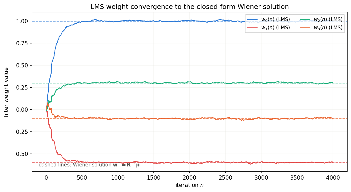
First, the closed-form Wiener solution \(w^*=[0.9989, -0.5984, 0.3015, -0.1022]\) computed via Eq.(4) is nearly identical to the true value \(h_{\text{true}}=[1.0, -0.6, 0.3, -0.1]\) , and \(J_{\min}=0.010337\) is almost exactly the measurement-noise variance \(\sigma_v^2=0.01\) (confirming, as predicted by Eq.(5), that the achievable minimum error equals the noise floor). And LMS — which never explicitly computed \(R\) or \(p\) — converges to a final weight vector \([1.0006, -0.5947, 0.3051, -0.1077]\) whose Euclidean distance from the Wiener solution is only \(7.7\times10^{-3}\) .
Tracking the weight error \(\|W_k - W^o\|\) over iterations makes the convergence process even clearer.
| Iteration \(k\) | \(\|W_k - W^o\|\) |
|---|---|
| 50 | 0.81228 |
| 100 | 0.51381 |
| 200 | 0.19565 |
| 500 | 0.01374 |
| 1000 | 0.01389 |
| 2000 | 0.01747 |
| 4000 | 0.00769 |
Starting from \(W_0=0\) , LMS rapidly approaches the neighborhood of the Wiener solution within a few hundred iterations, then continues to fluctuate around a residual error of order \(10^{-2}\) (excess MSE / misadjustment, caused by the noise in the instantaneous gradient) rather than converging exactly to zero. This residual fluctuation is an inherent property of LMS — a smaller step size \(\eta\) reduces it but slows convergence, a tradeoff whose quantitative theory (together with the convergence condition on the step size) is covered in LMS / NLMS Algorithms: Theory and Python Implementation .
Edge Case 3: The Limits of the Wiener Solution Under Non-Stationarity, and Tracking with LMS
The Wiener solution \(W^o=R^{-1}p\) in Eq.(4) implicitly assumes the input/desired-signal statistics (\(R, p\) ) are time-invariant (stationary). But many real-world systems (acoustic echo paths, fading communication channels, etc.) change over time (non-stationary), in which case a “fixed Wiener solution computed once” is no longer optimal after the statistics change. Adaptive algorithms like LMS, by contrast, keep updating their coefficients and can potentially track such changes. We verify this on a system-identification problem in which the unknown system abruptly changes partway through.
import numpy as np

np.random.seed(7)
N = 6000
M = 4
change_point = N // 2  # abrupt system change at n=3000

x = np.random.randn(N)
h1 = np.array([1.0, -0.6, 0.3, -0.1])
h2 = np.array([-0.5, 0.8, -0.4, 0.2])  # different system after the change
v = np.random.randn(N) * 0.1

d = np.zeros(N)
for n in range(M - 1, N):
    xv = x[n - M + 1 : n + 1][::-1]
    h = h1 if n < change_point else h2
    d[n] = h @ xv + v[n]

def build_R_p(x, d, M, n0, n1):
    X = np.zeros((n1 - n0, M))
    dd = np.zeros(n1 - n0)
    for k, n in enumerate(range(n0, n1)):
        X[k] = x[n - M + 1 : n + 1][::-1]
        dd[k] = d[n]
    R = (X.T @ X) / X.shape[0]
    p = (X.T @ dd) / X.shape[0]
    return R, p

# "fixed Wiener solution" computed only from pre-change data
R1, p1 = build_R_p(x, d, M, M - 1, change_point)
w_fixed = np.linalg.solve(R1, p1)
print("Fixed Wiener solution (pre-change data only) w_fixed =", np.array2string(w_fixed, precision=4))
print("h1 =", h1, " h2 =", h2)

# apply the fixed solution over the whole signal (both halves)
e_fixed = np.zeros(N)
for n in range(M - 1, N):
    xv = x[n - M + 1 : n + 1][::-1]
    e_fixed[n] = d[n] - w_fixed @ xv

# adaptive LMS run over the whole signal
mu = 0.02
w = np.zeros(M)
e_lms = np.zeros(N)
for n in range(M - 1, N):
    xv = x[n - M + 1 : n + 1][::-1]
    e_lms[n] = d[n] - w @ xv
    w = w + mu * e_lms[n] * xv

seg_pre = slice(M - 1, change_point)
seg_post_early = slice(change_point, change_point + 500)
seg_post_late = slice(N - 500, N)

for name, e in [("fixed-Wiener", e_fixed), ("LMS", e_lms)]:
    mse_pre = np.mean(e[seg_pre] ** 2)
    mse_early = np.mean(e[seg_post_early] ** 2)
    mse_late = np.mean(e[seg_post_late] ** 2)
    print(f"{name:12s}: MSE pre-change={mse_pre:.5f}  MSE post-change(early,500)={mse_early:.5f}  "
          f"MSE post-change(late,500)={mse_late:.5f}")

print(f"\nLMS final w(N) = {np.array2string(w, precision=4)}")
print(f"||w_LMS(N) - h2|| = {np.linalg.norm(w - h2):.5f}")
print(f"||w_fixed - h2||  = {np.linalg.norm(w_fixed - h2):.5f}")
Output:
Fixed Wiener solution (pre-change data only) w_fixed = [ 1.0011 -0.5988  0.3002 -0.0979]
h1 = [ 1.  -0.6  0.3 -0.1]  h2 = [-0.5  0.8 -0.4  0.2]
fixed-Wiener: MSE pre-change=0.00966  MSE post-change(early,500)=4.34709  MSE post-change(late,500)=5.09337
LMS         : MSE pre-change=0.02295  MSE post-change(early,500)=0.25829  MSE post-change(late,500)=0.01016

LMS final w(N) = [-0.5012  0.8011 -0.3913  0.1942]
||w_LMS(N) - h2|| = 0.01060
||w_fixed - h2||  = 2.18833
The fixed Wiener solution \(w_{\text{fixed}}=[1.0011, -0.5988, 0.3002, -0.0979]\) , computed from pre-change data, is nearly identical to \(h_1\) and achieves an MSE of \(0.00966\) (essentially the noise floor \(0.01\) , the theoretical optimum) in the pre-change segment. But once the system abruptly changes to \(h_2\) , \(w_{\text{fixed}}\) remains \(\|w_{\text{fixed}}-h_2\|=2.188\) away from \(h_2\) , and its MSE stays elevated at \(4.347\) immediately after the change and \(5.093\) even long after — the fixed solution never improves on its own.
Adaptive LMS (\(\mu=0.02\) ), by contrast, has a slightly worse pre-change MSE of \(0.02295\) (due to its inherent residual error), but although its MSE spikes temporarily to \(0.258\) right after the change, continuous coefficient updates let it re-learn \(h_2\) , and by the last 500 samples its MSE has recovered to \(0.01016\) — essentially the noise floor again. Its final weights, \(\|w_{\text{LMS}}(N)-h_2\|=0.0106\) , also match \(h_2\) almost exactly.
This result quantitatively demonstrates the essential difference, in a non-stationary environment, between “a Wiener solution computed once” and “an adaptive filter that keeps updating.” The Wiener solution is only optimal for the statistics at one instant, and does not automatically track an environment whose statistics keep changing. The real reason adaptive filters are chosen in practice is not merely that they can “learn to approximate” the Wiener solution — it is that they can chase the Wiener solution when it itself moves over time.
![]()
Recent Research
The theory of the Wiener-Hopf equation and MMSE linear filtering was established over half a century ago, but how to handle its ill-conditioning and its modern applications remain active research areas.
- Automatic determination of regularization: Zanco, Szczecinski, & Benesty (2023/2024, arXiv:2312.06560) propose a Bayesian statistical framework that automatically determines the regularization parameter \(\lambda\) from the observed signal itself, for the ridge regularization of an ill-conditioned \(R\) that we used in Edge Case 1 above, achieving near-optimal performance in system-identification and beamforming applications. Determining \(\lambda\) in a data-driven way, instead of a manual grid search, is a direct extension of the experiment in this article.
- A unified view of the Wiener solution, Kalman filtering, and LMS/NLMS: Szczecinski, Benesty, & Kuhn (2025, arXiv:2502.18325) re-derive adaptive filters from the framework of Bayesian sequential inference, showing that LMS, NLMS, and the Kalman filter emerge naturally under a Gaussian noise assumption, while robust variants such as the sign-error algorithm emerge under non-Gaussian (e.g. Laplacian) noise. This offers a broader statistical lens on Edge Case 2 above (what LMS is converging toward, and why).
- Re-evaluating the classical Wiener filter: Bled & Pitié (2023, arXiv:2303.16640) show that a carefully optimized implementation of the Wiener filter for image denoising can match the performance of deep-learning-based methods such as DnCNN — evidence that linear MMSE theory over half a century old remains practically relevant even in the era of deep learning.
Related Articles
- Fundamentals of Filtering Methods in Signal Processing - Systematic overview of Kalman filter, EKF, UKF, and particle filter.
- Frequency Characteristics of the EMA Filter - Frequency response of the EMA filter (a 1st-order IIR) visualized in Python.
- Lowpass Filter Design and Comparison - Compares moving average, Butterworth, and Chebyshev frequency responses.
- FIR vs IIR Filters: A Comprehensive Comparison - Systematic comparison of the two main digital filter classes (FIR / IIR) in characteristics and design philosophy.
- Chebyshev Filter Design: Theory and Python Implementation - Equiripple IIR filter — design and Python implementation of Type I and Type II.
- Bessel Filter: Theory and Python Implementation - IIR filter with maximally flat group delay; ideal when minimizing phase distortion.
- Bandpass Filter Design: Theory and Python Implementation - Band-pass design via lowpass + highpass composition and frequency transformation, with implementation examples.
- Wiener Filter: Optimal Linear Filtering Theory and Python Implementation - Extends this article’s Wiener-Hopf equation to the frequency domain (SNR-based gain design), and goes further into causality constraints, regularization for an ill-conditioned \(R\) , and the numerical equivalence to the Kalman filter.
- Adaptive Filters (LMS/RLS): Theory and Python Implementation - Builds on this article’s Wiener-Hopf equation and steepest descent to compare LMS, NLMS, and RLS with a noise-cancellation application.
- LMS / NLMS Algorithms: Theory and Python Implementation - A deeper follow-up on this article’s LMS algorithm, with rigorous proofs of the convergence condition and quantification of misadjustment.
- The RLS Algorithm in Python: Recursive Least Squares and Its Equivalence to the Kalman Filter - Covers the RLS algorithm, which solves this article’s Wiener-Hopf normal equation exactly and recursively via the matrix inversion lemma, and its numerical equivalence to the Kalman filter.
References
- Omatsu, S., “Signal Processing - Digital Filters”
- Haykin, S. (2014). Adaptive Filter Theory (5th ed.). Pearson. Chapters 1-2.
- Widrow, B., & Stearns, S. D. (1985). Adaptive Signal Processing. Prentice-Hall.
- Zanco, D. G. P., Szczecinski, L., & Benesty, J. (2023/2024). Automatic Regularization for Linear MMSE Filters. arXiv:2312.06560. https://arxiv.org/abs/2312.06560
- Szczecinski, L., Benesty, J., & Kuhn, E. V. (2025). A Unified Bayesian Perspective for Conventional and Robust Adaptive Filters. arXiv:2502.18325. https://arxiv.org/abs/2502.18325
- Bled, C., & Pitié, F. (2023). Pushing The Limits of the Wiener Filter in Image Denoising. arXiv:2303.16640. https://arxiv.org/abs/2303.16640