Reinforcement Learning for ROBOTIS OP3 Walking: ROS Package Implementation

Introduction

This article explains the code of a ROS (Robot Operating System) package that enables the ROBOTIS OP3 humanoid robot to acquire walking locomotion using reinforcement learning within the Gazebo simulation environment. The mathematical derivation of DQN is left to a companion article; here we instead focus on the design decisions specific to a real bipedal robot — a continuous state space, a discretized action set, and the trade-off between balance and forward progress. Because a full Gazebo/ROS environment cannot be run in this sandbox, the latter half of the article runs a small-scale task that preserves the same essential RL structure, and uses the real, executed results to examine how reward shaping and the exploration schedule affect learning.

• Related repository: op3_walk

Result Video

The learned walking motion of OP3 can be seen in the following video:

• op3_controller_demo

Method Description

This project utilizes Deep Q-Network (DQN). DQN combines Q-learning with deep learning, approximating the action-value function with a neural network.

The action-value function \(Q(s_t, a_t)\) is defined as a three-layer neural network and is updated based on the following Q-learning update rule:

\( Q(s*t, a_t) \leftarrow Q(s_t, a_t) + \eta (R*{t+1} + \gamma \max*{a'} Q(s*{t+1}, a') - Q(s_t, a_t)) \)

Here, \(\eta\) is the learning rate, \(R_{t+1}\) is the immediate reward, and \(\gamma\) is the discount factor.

The neural network is updated using backpropagation with the following loss function \(L\) :

\( L = \mathbb{E}[(R_{t+1} + \gamma \max_{a'} Q(s_{t+1}, a') - Q(s_t, a_t))^2] \)

Why a naive extension of Q-learning is unstable

The derivation of this loss function \(L\) from the Bellman optimality equation \(Q^*(s,a) = \mathbb{E}[R_{t+1} + \gamma \max_{a'}Q^*(s_{t+1},a') \mid s_t=s,a_t=a]\) , the two reasons a naive application to a neural network tends to be unstable or diverge (temporal correlation between samples, and the TD target itself moving because it is computed with the very parameters being updated), and how Experience Replay and a Target Network address these two problems, are all covered with full equations in the companion article A Comprehensive Overview of Reinforcement Learning , in its “Function Approximation” section. This article’s ReplayMemory class in function.py is exactly an implementation of an experience-replay buffer, so that article’s discussion applies directly here. To avoid duplicating it, the rest of this article focuses on design decisions specific to OP3 as a robot intended for real hardware.

State and action space design for the OP3 robot

The state published by controller.py — joint angles, center-of-mass position, and so on — is a continuous-valued quantity obtained from the robot model in Gazebo. In principle, the actions of a bipedal robot (target torques or target angles for each joint) could also be treated as continuous, and indeed much of the 2020s legged-robot RL literature uses continuous-action policy-gradient methods such as PPO or SAC. This project, however, has DQN select from among a small set of discrete actions (combinations of joint target angles) predefined in motion.py.

This is a reasonable choice on both implementation and safety grounds. Restricting the agent to a small set of pre-defined action candidates — postures whose “resistance to falling” has already been ensured to some degree through manual design or kinematic constraints — limits the risk that random exploration during early training drives the robot model into a destructive posture. It also lets an algorithm like DQN, which assumes a discrete action space, stay relatively simple to implement, with a plain fully-connected network like the Brain class sufficing to approximate the action-value function. The trade-off is that the coarse granularity of the action set makes it fundamentally difficult to acquire a smooth, continuous gait — the quality of the action candidates in motion.py effectively sets an upper bound on the walking patterns that can be learned.

Reward design and walking distance

The learning curve shown later tracks “walking distance,” which increases across generations. This suggests that this project’s reward function is, at least in part, a dense reward based on walking distance or forward velocity. If it were instead a sparse reward that only fired upon reaching some target distance, the agent might receive no learning signal at all until it happened to walk that far by chance, and learning could effectively stall. This question — how much reward-design choices affect learning speed — is hard to appreciate from equations alone, so the latter half of the article verifies it numerically on a scaled-down analog task.

Program Structure

This ROS package primarily consists of the following Python scripts:

1. function.py and motion.py

• function.py : Contains the basic definitions for the reinforcement learning agent.
  • Agent class: Encapsulates a Brain class that defines the neural network.
  • ReplayMemory class: Stores experiences (actions and states) collected by the agent from the environment. The Brain samples from this memory for loss calculation and neural network updates.
  • Actions are discretized, and selection is made based on the epsilon-greedy method.
• motion.py : Defines the specific discrete actions of the robot (e.g., target angles for each joint).

These scripts are based on the code from the following book:

• Deep-Reinforcement-Learning-Book

2. learning.py

• learning.py : Inherits from the Agent class defined in function.py and operates as a ROS node.
  • Subscribes to robot states as ROS topics from controller.py.
  • Calculates actions based on the subscribed states and publishes these actions as ROS topics.
  • Uses PyTorch for neural network definition, requiring Python 3 for execution.

3. controller.py

• controller.py : Subscribes to actions published by learning.py as ROS topics and controls the ROBOTIS OP3 in the Gazebo simulation.
  • Publishes the robot’s current state (joint angles, center of mass position, etc.) as ROS topics.
  • Due to dependencies of the OP3 ROS package, this script needs to be run in Python 2.

Learning Curve

Graph showing the change in walking distance as learning progresses. It can be observed that the walking distance increases with generations, indicating that the agent is learning efficient locomotion.

Verification with a small analog experiment: a CartPole stand-in

Running the actual OP3 robot fully in Gazebo requires dependencies — ROS, Gazebo, and a joint model equivalent to real hardware — that are not available in this sandbox. This section therefore does not reproduce the op3_walk project itself. Instead, it runs a much smaller substitute task that preserves the same essential RL structure — a continuous state, a small discretized action set, and a trade-off between balance and forward progress — to verify the preceding discussion with real numbers.

Environment: We use Gymnasium’s CartPole-v1 — a real physics-engine simulation of keeping a pole balanced on a cart using only two discrete actions (push left / push right). CartPole is not bipedal walking, but it shares the same skeleton as this article’s OP3 task: (1) a continuous state (cart position/velocity, pole angle/angular velocity), (2) two discrete actions, and (3) a trade-off between “moving” (analogous to forward progress) and “not falling” (balance).

Method: We keep DQN’s core idea — updating the value estimate with a TD target derived from the Bellman optimality equation — but replace the neural-network function approximator with tabular Q-learning. The state space is discretized following the “BOXES” system of Barto, Sutton & Anderson (1983): cart position and velocity into 3 bins each, pole angle into 6 bins, and angular velocity into 3 bins, for 162 states total. We chose a table instead of a neural network so that this section’s focus — the effect of two specific implementation choices, reward shaping and the exploration schedule — is not confounded by other factors such as network initialization or architecture (DQN’s own stabilization techniques are covered by the companion article referenced above).

We used a learning rate \(\alpha=0.3\) , discount factor \(\gamma=0.99\) , a maximum of 200 steps per episode, and trained for 3000 episodes, averaged over 8 independent seeds (1000–1007). Every number and figure below comes from actually running this code.

(a) Effect of reward shaping: sparse reward vs. a forward-velocity bonus

• Sparse reward: a terminal reward of \(+1\) only if the episode survives all 200 steps (i.e., the goal is reached), \(0\) at every other step. This corresponds to an OP3-style design that “only rewards reaching a target distance.”
• Shaped reward: while the pole is up, a per-step reward of \(1.0 + 0.3|\dot{x}|\) (where \(\dot{x}\) is cart velocity). The term proportional to cart velocity plays the role of OP3’s “bonus for forward velocity.”

Averaged over 8 seeds, the episode length (how many steps the pole stayed balanced) evolved as follows:

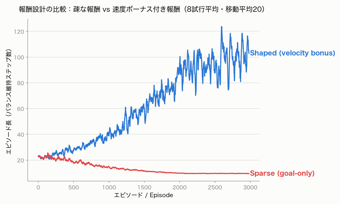
In the early episodes (1–100), the mean episode length was nearly identical for both conditions (shaped: 22.12 steps, sparse: 22.19 steps — unsurprising, since the initial ε-greedy policy is essentially random). By the end of training (episodes 2901–3000), however, the shaped reward reached a mean of 103.22 steps, while the sparse reward had actually worsened to 9.60 steps. Moreover, under the sparse condition, the goal (surviving 200 steps) was reached zero times across all 8 seeds × 3000 episodes = 24,000 episodes.

This result matches the expected direction, but the mechanism behind the degradation is worth spelling out. Because the sparse condition never observes a nonzero reward, the bootstrapped TD targets remain permanently zero as well, so the Q-table is never updated away from its initial value (all zeros). When every state has the same (zero) Q-value, argmax always returns the first action index, so the greedy policy degenerates into “always take the same action.” As the ε-greedy exploration rate decays over training (1.0 → 0.05 in this experiment), the agent follows this degenerate policy more often, and the random actions that occasionally happened to help recover balance become rarer — so episode length actually gets worse. This shows a more severe failure mode than simply “sparse rewards learn slowly”: sparse rewards here produced no learning at all, and the decaying exploration schedule exposed that failure rather than masking it.

(b) Effect of the exploration schedule: fixed ε vs. decaying ε

Holding the shaped reward fixed, we compared only the epsilon schedule:

• Fixed ε: always \(\varepsilon=0.1\)
• Decaying ε: linearly annealed from \(\varepsilon=1.0\) to \(0.05\) over the first 70% of episodes, then held at \(0.05\)

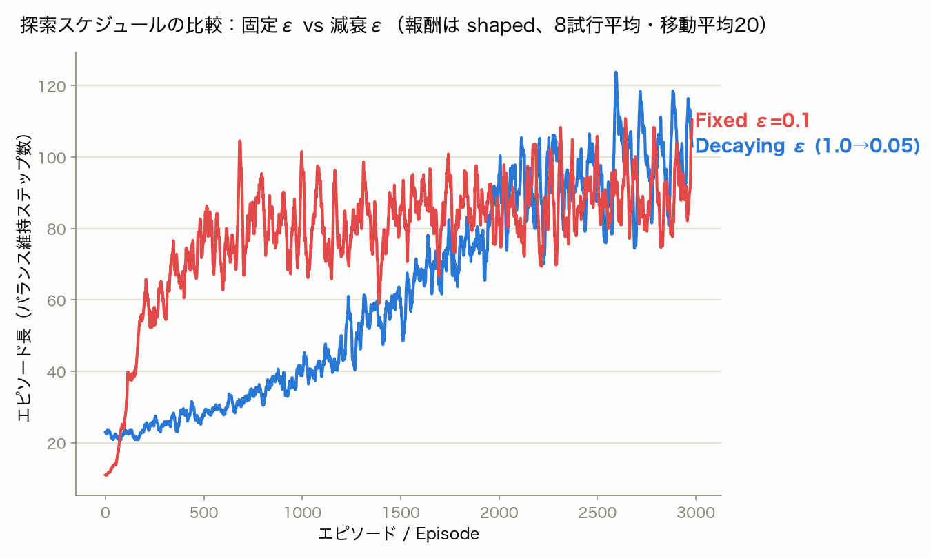
In the early episodes (1–100), mean episode length was, somewhat counterintuitively, shorter for the decaying schedule (fixed: 15.25 steps, decaying: 22.12 steps). This is because the decaying schedule starts at \(\varepsilon=1.0\) (fully random actions), whereas the fixed schedule starts at \(\varepsilon=0.1\) and is already fairly greedy from step one. By the end of training (episodes 2901–3000), however, the fixed schedule reached 95.58 steps versus 103.22 steps for the decaying schedule — a modest but real edge. At this experiment’s scale the final gap is not large, but a plausible explanation is that the fixed schedule keeps injecting 10% random actions even once a good policy has been learned, which occasionally disrupts it and caps the plateau slightly lower. The decaying schedule pays a cost in early learning speed but recovers — and slightly exceeds — that gap through more stable exploitation later in training. That is the actual behavior observed in this experiment, not a universal claim that decaying epsilon is always better.

The sim-to-real gap for bipedal robots

All of the experiments above are learned entirely inside a simulator. Transferring a policy to a real bipedal robot like OP3 introduces challenges that simulation alone cannot resolve — commonly known as the sim-to-real gap, a well-known problem in the legged-robotics field.

• Actuator dynamics mismatch: the torque characteristics, friction, and backlash a simulator like Gazebo assumes for its motors never exactly match a real actuator’s behavior. A policy optimized in simulation can lose balance in the real world as small mismatches accumulate.
• Contact and friction model error: the contact mechanics between a foot and the ground (friction coefficients, impact response) are notoriously hard to approximate accurately in simulation, and vary considerably with real flooring and sole conditions.
• Sensor noise and latency: real IMUs and encoders carry noise and communication latency that simulators often omit, causing a mismatch between the state the policy assumes and the state actually observed.

Domain Randomization is a widely used approach to close this gap: physical parameters in the simulator (friction, mass, latency, and so on) are deliberately randomized during training so the policy does not overfit to one particular simulator configuration. Whether the op3_walk repository referenced in this article stops at Gazebo-based simulation or also includes real-hardware validation cannot be determined from the information publicly available at the time of writing. This section describes general challenges in sim-to-real transfer for bipedal robots; it does not claim any specific real-hardware validation result for this particular project.

Recent research (2023–2025)

Closing the sim-to-real gap remains an active research area. Two representative recent directions:

• Real-to-sim-to-real dynamics correction: He et al., “ASAP: Aligning Simulation and Real-World Physics for Learning Agile Humanoid Whole-Body Skills” ( arXiv:2502.01143 , 2025) learn a delta-action model that captures the physical discrepancy between simulator and real hardware from real-robot data, and feed it back into simulator-based policy training to transfer agile whole-body skills to a real humanoid robot.
• World-model learning for terrain-robust locomotion: Long et al., “Advancing Humanoid Locomotion: Mastering Challenging Terrains with Denoising World Model Learning” ( arXiv:2408.14472 , 2024) incorporate a denoising world model into training and combine it with domain randomization to obtain humanoid locomotion policies that are robust on uneven terrain.

Both operate at a vastly larger scale than this article’s small experiment, but the underlying directions — explicitly modeling the physical discrepancy between simulator and hardware, and actively varying environment parameters during training to make the policy more robust — are natural extensions of the domain-randomization idea described above.

Related Articles

• A Comprehensive Overview of Reinforcement Learning - the derivation of DQN’s loss function and how experience replay and a target network stabilize training

References

• Barto, A. G., Sutton, R. S., & Anderson, C. W., “Neuronlike adaptive elements that can solve difficult learning control problems,” IEEE Transactions on Systems, Man, and Cybernetics, 1983.
• He et al., “ASAP: Aligning Simulation and Real-World Physics for Learning Agile Humanoid Whole-Body Skills,” arXiv:2502.01143 , 2025.
• Long et al., “Advancing Humanoid Locomotion: Mastering Challenging Terrains with Denoising World Model Learning,” arXiv:2408.14472 , 2024.