SQL has a lot of syntax to keep straight, and things like “the four kinds of JOIN,” “when to use WHERE vs. HAVING,” and “how window functions are written” are exactly the kind of thing people re-search every time they need them. This article is a reference cheat sheet that uses just two consistent sample tables (employees and departments) to walk through everything from basic SELECT to subqueries and window functions, always as a “query + result” pair you can check at a glance. The syntax follows standard SQL, with dialect notes only where MySQL and PostgreSQL genuinely diverge.
1. Setting Up the Sample Tables
Every example below runs against these two tables: employees (7 rows) and departments (4 rows). I’ve deliberately mixed in “an employee with no department assigned” (Frank) and “a department with no employees” (HR) — that’s what makes the differences between JOIN types and subqueries visible.
CREATE TABLE departments (
    dept_id   INTEGER PRIMARY KEY,
    dept_name TEXT NOT NULL,
    location  TEXT NOT NULL
);

CREATE TABLE employees (
    emp_id    INTEGER PRIMARY KEY,
    name      TEXT NOT NULL,
    dept_id   INTEGER REFERENCES departments(dept_id),
    salary    INTEGER NOT NULL,
    hire_year INTEGER NOT NULL
);

INSERT INTO departments (dept_id, dept_name, location) VALUES
  (1, 'Engineering', 'Tokyo'),
  (2, 'Sales',       'Osaka'),
  (3, 'Marketing',   'Tokyo'),
  (4, 'HR',          'Fukuoka');

INSERT INTO employees (emp_id, name, dept_id, salary, hire_year) VALUES
  (101, 'Alice', 1,    720000, 2019),
  (102, 'Bob',   2,    580000, 2020),
  (103, 'Carol', 1,    810000, 2018),
  (104, 'Dave',  3,    540000, 2021),
  (105, 'Eve',   2,    610000, 2022),
  (106, 'Frank', NULL, 500000, 2023),
  (107, 'Grace', 1,    690000, 2021);
departments
| dept_id | dept_name | location |
|---|---|---|
| 1 | Engineering | Tokyo |
| 2 | Sales | Osaka |
| 3 | Marketing | Tokyo |
| 4 | HR | Fukuoka |
employees
| emp_id | name | dept_id | salary | hire_year |
|---|---|---|---|---|
| 101 | Alice | 1 | 720000 | 2019 |
| 102 | Bob | 2 | 580000 | 2020 |
| 103 | Carol | 1 | 810000 | 2018 |
| 104 | Dave | 3 | 540000 | 2021 |
| 105 | Eve | 2 | 610000 | 2022 |
| 106 | Frank | NULL | 500000 | 2023 |
| 107 | Grace | 1 | 690000 | 2021 |
Frank has not been assigned a department yet (dept_id is NULL), and nobody has been assigned to HR yet (dept_id = 4) — both deliberately.
2. SELECT Basics — Choosing Columns and WHERE
Selecting columns
SELECT name, salary FROM employees;
This pulls just name and salary from the 7 rows in employees. The row count doesn’t change — still 7 rows.
Filtering with comparison operators
SELECT name, salary FROM employees WHERE salary >= 600000;
| name | salary |
|---|---|
| Alice | 720000 |
| Carol | 810000 |
| Eve | 610000 |
| Grace | 690000 |
Combining conditions with AND / OR
SELECT name, dept_id, salary FROM employees
WHERE dept_id = 1 AND salary >= 700000;
| name | dept_id | salary |
|---|---|---|
| Alice | 1 | 720000 |
| Carol | 1 | 810000 |
AND keeps rows that satisfy both conditions; OR keeps rows that satisfy either one. AND binds tighter than OR, so when you mix them, it’s safer to make the grouping explicit with parentheses, e.g. (dept_id = 1 OR dept_id = 3) AND salary >= 700000.
Pattern matching with LIKE
SELECT name FROM employees WHERE name LIKE 'A%';   -- prefix match
SELECT name FROM employees WHERE name LIKE '%e';    -- suffix match
'A%' (starts with A) matches only Alice. '%e' (ends with e) matches Alice, Dave, and Eve — 3 rows. % is a wildcard for zero or more characters, and _ matches exactly one character.
Matching a list with IN
SELECT name, dept_id FROM employees WHERE dept_id IN (1, 3);
| name | dept_id |
|---|---|
| Alice | 1 |
| Carol | 1 |
| Dave | 3 |
| Grace | 1 |
This means the same thing as dept_id = 1 OR dept_id = 3, but IN reads more cleanly once you have several candidates.
Range checks with BETWEEN
SELECT name, salary FROM employees
WHERE salary BETWEEN 550000 AND 700000;
| name | salary |
|---|---|
| Bob | 580000 |
| Eve | 610000 |
| Grace | 690000 |
BETWEEN A AND B is equivalent to salary >= A AND salary <= B — a closed interval that includes both endpoints.
Checking for NULL
SELECT name FROM employees WHERE dept_id IS NULL;
| name |
|---|
| Frank |
NULL represents “no value present,” a special state that = NULL can never match. Always use IS NULL / IS NOT NULL.
3. Sorting and Limiting Row Counts
ORDER BY
SELECT name, salary FROM employees ORDER BY salary DESC;
| name | salary |
|---|---|
| Carol | 810000 |
| Alice | 720000 |
| Grace | 690000 |
| Eve | 610000 |
| Bob | 580000 |
| Dave | 540000 |
| Frank | 500000 |
You can specify ASC (ascending, the default) or DESC (descending). With multiple columns, the leftmost key takes priority.
SELECT name, dept_id, salary FROM employees
ORDER BY dept_id ASC, salary DESC;
| name | dept_id | salary |
|---|---|---|
| Carol | 1 | 810000 |
| Alice | 1 | 720000 |
| Grace | 1 | 690000 |
| Eve | 2 | 610000 |
| Bob | 2 | 580000 |
| Dave | 3 | 540000 |
| Frank | NULL | 500000 |
Within each dept_id group, salary DESC takes over. NULL placement is a dialect difference: PostgreSQL puts NULLs last by default for ASC, while MySQL puts them first (the table above follows PostgreSQL’s default). If you need precise control, use NULLS LAST / NULLS FIRST (standard SQL, supported by PostgreSQL).
Limiting rows with LIMIT / OFFSET
SELECT name, salary FROM employees
ORDER BY salary DESC
LIMIT 3;
| name | salary |
|---|---|
| Carol | 810000 |
| Alice | 720000 |
| Grace | 690000 |
SELECT name, salary FROM employees
ORDER BY salary DESC
LIMIT 3 OFFSET 3;
| name | salary |
|---|---|
| Eve | 610000 |
| Bob | 580000 |
| Dave | 540000 |
This skips the first 3 rows and takes the next 3 — the basic pattern behind pagination. LIMIT/OFFSET is common to MySQL, PostgreSQL, and SQLite, but standard SQL uses FETCH FIRST 3 ROWS ONLY and SQL Server uses TOP 3 — worth remembering as a dialect difference.
4. Aggregation and Grouping — GROUP BY / HAVING
Aggregate functions
SELECT COUNT(*) AS cnt, SUM(salary) AS total,
       AVG(salary) AS avg_salary, MAX(salary) AS max_salary, MIN(salary) AS min_salary
FROM employees;
| cnt | total | avg_salary | max_salary | min_salary |
|---|---|---|---|---|
| 7 | 4450000 | 635714.29… | 810000 | 500000 |
COUNT(*) counts rows, and AVG divides the sum by the row count (4,450,000 ÷ 7 ≈ 635,714.29). If you specify a column, e.g. COUNT(dept_id), rows where that column is NULL (Frank) get excluded from the count.
GROUP BY
SELECT dept_id, COUNT(*) AS cnt, AVG(salary) AS avg_salary
FROM employees
GROUP BY dept_id;
| dept_id | cnt | avg_salary |
|---|---|---|
| 1 | 3 | 740000.00 |
| 2 | 2 | 595000.00 |
| 3 | 1 | 540000.00 |
| NULL | 1 | 500000.00 |
GROUP BY collects rows with the same value in the given column into one group, then computes the aggregate functions in SELECT per group. NULL forms its own group too (a “NULL group” containing just Frank).
HAVING — filtering groups
SELECT dept_id, COUNT(*) AS cnt
FROM employees
GROUP BY dept_id
HAVING COUNT(*) >= 2;
| dept_id | cnt |
|---|---|
| 1 | 3 |
| 2 | 2 |
Both dept_id = 3 and the NULL group have only 1 member, so HAVING drops them.
The difference between WHERE and HAVING comes down to which stage they filter at. WHERE filters individual rows before aggregation; HAVING filters the resulting groups after GROUP BY. Using both together looks like this:
SELECT dept_id, AVG(salary) AS avg_salary
FROM employees
WHERE dept_id IS NOT NULL
GROUP BY dept_id
HAVING AVG(salary) >= 600000;
| dept_id | avg_salary |
|---|---|
| 1 | 740000.00 |
The order of operations is: WHERE first excludes Frank (NULL department), the remaining 6 rows get grouped by dept_id, and then HAVING keeps only groups whose average salary is at least 600,000. Department 2 (average 595,000) falls short and drops out. It’s also worth remembering that HAVING can reference aggregate functions like COUNT(*) or AVG(salary), while WHERE cannot — at the WHERE stage, aggregate values don’t exist yet.
5. JOIN — Combining Multiple Tables
Here we join employees and departments on dept_id. Depending on the type of join, Frank (no department) and HR (no employees) get treated differently.
SELECT e.name, d.dept_name, d.location
FROM employees AS e
INNER JOIN departments AS d ON e.dept_id = d.dept_id;
INNER JOIN (only matched rows, 6 rows)
| name | dept_name | location |
|---|---|---|
| Alice | Engineering | Tokyo |
| Bob | Sales | Osaka |
| Carol | Engineering | Tokyo |
| Dave | Marketing | Tokyo |
| Eve | Sales | Osaka |
| Grace | Engineering | Tokyo |
Neither Frank (no department) nor HR (no employees) has a matching partner, so neither appears in the result at all.
SELECT e.name, d.dept_name
FROM employees AS e
LEFT JOIN departments AS d ON e.dept_id = d.dept_id;
LEFT JOIN (all of employees, plus matches, 7 rows)
| name | dept_name |
|---|---|
| Alice | Engineering |
| Bob | Sales |
| Carol | Engineering |
| Dave | Marketing |
| Eve | Sales |
| Frank | NULL |
| Grace | Engineering |
The left side (employees, listed in FROM) always survives in full. Frank has no matching department, so dept_name comes back NULL but Frank still appears. HR, which only ever existed on the right side, doesn’t show up at all.
SELECT e.name, d.dept_name
FROM employees AS e
RIGHT JOIN departments AS d ON e.dept_id = d.dept_id;
RIGHT JOIN (all of departments, plus matches, 7 rows)
| name | dept_name |
|---|---|
| Alice | Engineering |
| Carol | Engineering |
| Grace | Engineering |
| Bob | Sales |
| Eve | Sales |
| Dave | Marketing |
| NULL | HR |
This time it’s the right side (departments) that survives in full. HR has no employees, so name comes back NULL but HR still appears. Frank doesn’t, since his department doesn’t match anything.
SELECT e.name, d.dept_name
FROM employees AS e
FULL JOIN departments AS d ON e.dept_id = d.dept_id;
FULL JOIN (the union of both sides, 8 rows)
| name | dept_name |
|---|---|
| Alice | Engineering |
| Bob | Sales |
| Carol | Engineering |
| Dave | Marketing |
| Eve | Sales |
| Frank | NULL |
| Grace | Engineering |
| NULL | HR |
Both Frank and HR survive. Think of FULL JOIN as adding LEFT and RIGHT together and collapsing the overlap (the 6 matched rows) down to a single copy.
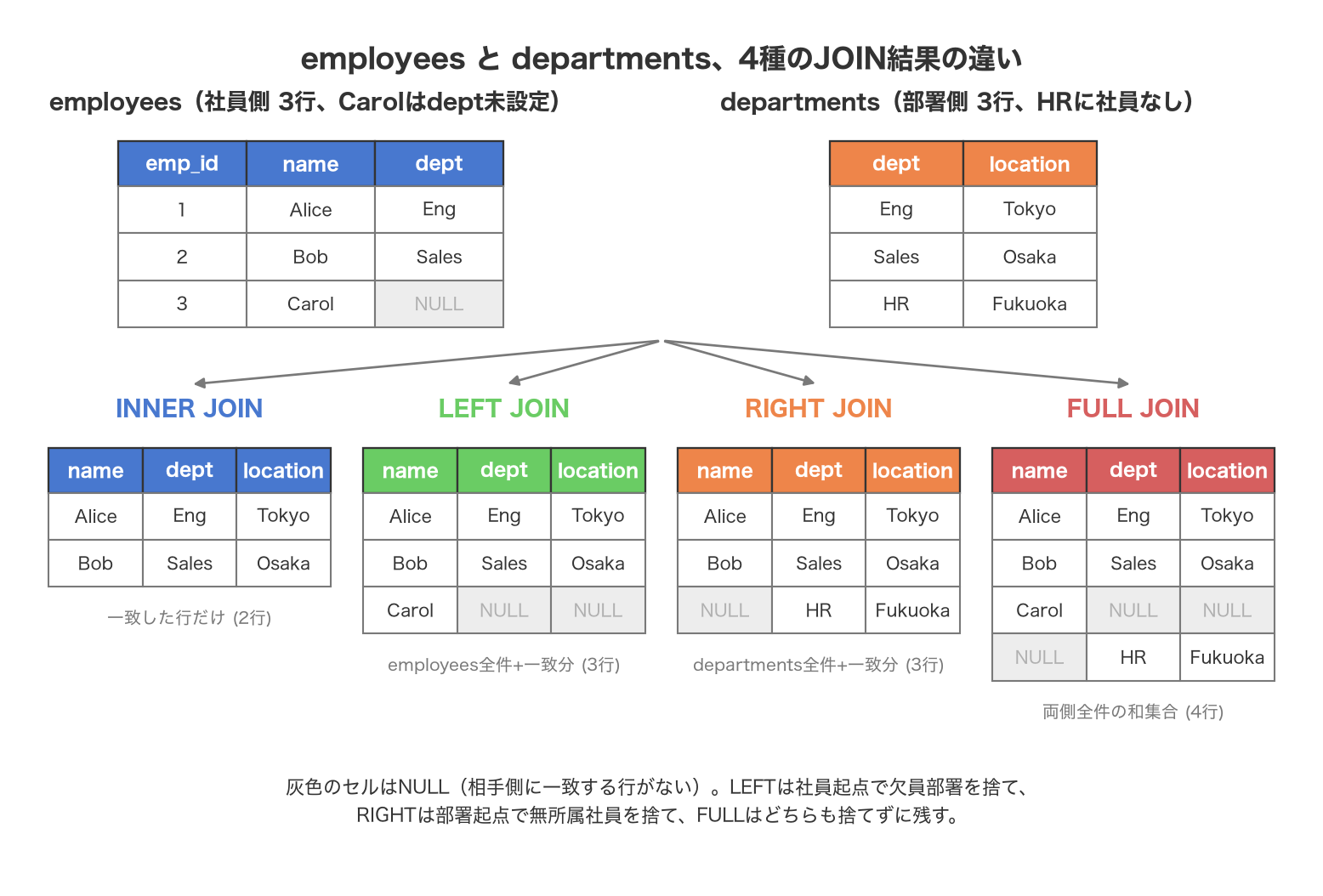
Why does a JOIN change the row count? Because a join is fundamentally an operation that enumerates every matching combination of rows from both tables. If a department has 3 employees, that department appears 3 times in the joined result — which is exactly why Engineering shows up 3 times. Rows with no matching partner disappear under INNER JOIN, but survive padded with NULL under LEFT, RIGHT, and FULL.
Note that MySQL doesn’t support FULL JOIN directly (PostgreSQL and SQL Server do). To get an equivalent result in MySQL, you need to combine a LEFT JOIN result with a RIGHT JOIN result via UNION.
6. Subqueries
A subquery inside WHERE
Find employees earning more than the average salary.
SELECT name, salary FROM employees
WHERE salary > (SELECT AVG(salary) FROM employees);
| name | salary |
|---|---|
| Alice | 720000 |
| Carol | 810000 |
| Grace | 690000 |
The inner query (SELECT AVG(salary) FROM employees) is evaluated first, collapsing to a single value (635714.29), which the outer query then uses like a constant. Eve (610000) falls below the average, so she’s excluded.
A subquery inside FROM (derived table)
First aggregate the average salary per department, then keep only departments averaging 600,000 or more.
SELECT dept_id, avg_salary
FROM (
    SELECT dept_id, AVG(salary) AS avg_salary
    FROM employees
    WHERE dept_id IS NOT NULL
    GROUP BY dept_id
) AS dept_avg
WHERE avg_salary >= 600000;
| dept_id | avg_salary |
|---|---|
| 1 | 740000.00 |
A subquery inside FROM is called a “derived table” — it lets you reuse an aggregation result as if it were an ordinary table. This gives the same result as HAVING in the previous section, but tends to read more naturally when you need to apply further processing on top of the aggregated result.
Correlated subqueries
Find employees earning more than the average salary within their own department. The key here is that the inner subquery (e2) references a row from the outer query (e1).
SELECT e1.name, e1.salary
FROM employees AS e1
WHERE e1.salary > (
    SELECT AVG(e2.salary)
    FROM employees AS e2
    WHERE e2.dept_id = e1.dept_id
);
| name | salary |
|---|---|
| Carol | 810000 |
| Eve | 610000 |
A correlated subquery re-evaluates for every single row of the outer query. Carol qualifies because 810,000 exceeds Engineering’s department average of 740,000; Alice and Grace fall short of that average and are excluded. Frank is excluded too — since his dept_id is NULL, the comparison e2.dept_id = e1.dept_id becomes NULL = NULL, which is always UNKNOWN (treated as false).
EXISTS / NOT EXISTS
Find departments that have at least one employee.
SELECT dept_name FROM departments AS d
WHERE EXISTS (
    SELECT 1 FROM employees AS e WHERE e.dept_id = d.dept_id
);
| dept_name |
|---|
| Engineering |
| Sales |
| Marketing |
To find departments with zero employees (i.e., vacant departments), use NOT EXISTS.
SELECT dept_name FROM departments AS d
WHERE NOT EXISTS (
    SELECT 1 FROM employees AS e WHERE e.dept_id = d.dept_id
);
| dept_name |
|---|
| HR |
EXISTS is a “does this exist” operator that becomes true as soon as the subquery returns even one row — it doesn’t look at the actual values. Many engines can stop searching the moment a match is found, which often makes EXISTS more efficient than an equivalent IN check.
7. Branching Logic with CASE
Classify salaries into three bands.
SELECT name, salary,
    CASE
        WHEN salary >= 700000 THEN 'High'
        WHEN salary >= 600000 THEN 'Mid'
        ELSE 'Standard'
    END AS salary_band
FROM employees
ORDER BY salary DESC;
| name | salary | salary_band |
|---|---|---|
| Carol | 810000 | High |
| Alice | 720000 | High |
| Grace | 690000 | Mid |
| Eve | 610000 | Mid |
| Bob | 580000 | Standard |
| Dave | 540000 | Standard |
| Frank | 500000 | Standard |
CASE evaluates conditions from top to bottom and returns the result of the first WHEN that’s true (falling through to ELSE if nothing matches). This form — a series of WHEN expression THEN value clauses — is called a “searched CASE expression.” There’s also a “simple CASE expression” written as CASE column WHEN value1 THEN ... WHEN value2 THEN ..., but the searched form above is better suited to range checks like this one.
CASE also pairs well with aggregate functions for “conditional counting.”
SELECT
    SUM(CASE WHEN salary >= 700000 THEN 1 ELSE 0 END) AS high_cnt,
    SUM(CASE WHEN salary >= 600000 AND salary < 700000 THEN 1 ELSE 0 END) AS mid_cnt,
    SUM(CASE WHEN salary < 600000 THEN 1 ELSE 0 END) AS standard_cnt
FROM employees;
| high_cnt | mid_cnt | standard_cnt |
|---|---|---|
| 2 | 2 | 3 |
This gets you per-band headcounts side by side in a single aggregated row, without using GROUP BY at all — a pattern that comes up constantly in dashboard queries.
8. Introduction to Window Functions
Unlike GROUP BY, window functions don’t collapse rows — they attach extra information, like a rank or a running total within the same group, to every row. The syntax is OVER (PARTITION BY ... ORDER BY ...).
ROW_NUMBER — salary rank within department
SELECT name, dept_id, salary,
    ROW_NUMBER() OVER (PARTITION BY dept_id ORDER BY salary DESC) AS rn
FROM employees
ORDER BY dept_id, rn;
| name | dept_id | salary | rn |
|---|---|---|---|
| Carol | 1 | 810000 | 1 |
| Alice | 1 | 720000 | 2 |
| Grace | 1 | 690000 | 3 |
| Eve | 2 | 610000 | 1 |
| Bob | 2 | 580000 | 2 |
| Dave | 3 | 540000 | 1 |
| Frank | NULL | 500000 | 1 |
PARTITION BY dept_id creates a separate “window” per department, and numbering restarts inside each window according to ORDER BY salary DESC. The crucial difference from GROUP BY is that all 7 original rows survive.
RANK — handling ties
SELECT name, salary,
    RANK() OVER (ORDER BY salary DESC) AS rnk
FROM employees
ORDER BY rnk;
| name | salary | rnk |
|---|---|---|
| Carol | 810000 | 1 |
| Alice | 720000 | 2 |
| Grace | 690000 | 3 |
| Eve | 610000 | 4 |
| Bob | 580000 | 5 |
| Dave | 540000 | 6 |
| Frank | 500000 | 7 |
Since every salary in this sample data is unique, RANK produces the same result as ROW_NUMBER here. The two only diverge when there are ties. For example, if two people tied for 1st place with the same salary, RANK would give both of them rank 1 and then skip straight to rank 3 for the next person (rank 2 is never used). If you don’t want that gap, use DENSE_RANK instead (both get rank 1, and the next person gets rank 2). Pick whichever of the three matches your use case.
SUM() OVER — attaching a total without collapsing rows
Attach each department’s total salary to every row, without reducing the row count.
SELECT name, dept_id, salary,
    SUM(salary) OVER (PARTITION BY dept_id) AS dept_total
FROM employees
ORDER BY dept_id;
| name | dept_id | salary | dept_total |
|---|---|---|---|
| Alice | 1 | 720000 | 2220000 |
| Carol | 1 | 810000 | 2220000 |
| Grace | 1 | 690000 | 2220000 |
| Bob | 2 | 580000 | 1190000 |
| Eve | 2 | 610000 | 1190000 |
| Dave | 3 | 540000 | 540000 |
| Frank | NULL | 500000 | 500000 |
This is handy when you want something like “what percentage of my department’s total salary do I earn” in a single query — much more concise than grouping and then joining back.
Adding ORDER BY inside the window also lets you build a running total.
SELECT name, salary,
    SUM(salary) OVER (ORDER BY salary DESC
        ROWS BETWEEN UNBOUNDED PRECEDING AND CURRENT ROW) AS running_total
FROM employees
ORDER BY salary DESC;
| name | salary | running_total |
|---|---|---|
| Carol | 810000 | 810000 |
| Alice | 720000 | 1530000 |
| Grace | 690000 | 2220000 |
| Eve | 610000 | 2830000 |
| Bob | 580000 | 3410000 |
| Dave | 540000 | 3950000 |
| Frank | 500000 | 4450000 |
You can confirm that the running total on the last row (4,450,000) matches the overall SUM(salary) computed back in section 4.
9. Modifying Data — INSERT / UPDATE / DELETE
INSERT — adding a row
INSERT INTO employees (emp_id, name, dept_id, salary, hire_year)
VALUES (108, 'Henry', 2, 550000, 2026);
Henry joins the Sales team (dept_id = 2), bringing employees to 8 rows.
UPDATE — modifying existing rows
Give everyone in Engineering (dept_id = 1) a 5% raise.
UPDATE employees
SET salary = salary * 1.05
WHERE dept_id = 1;
| name | salary (before) | salary (after) |
|---|---|---|
| Alice | 720000 | 756000 |
| Carol | 810000 | 850500 |
| Grace | 690000 | 724500 |
DELETE — removing rows
Remove employees who joined before 2019.
DELETE FROM employees WHERE hire_year < 2019;
Only Carol, with hire_year = 2018, matches — and she’s the one row that gets deleted.
Forgetting WHERE is the single most dangerous mistake you can make with UPDATE/DELETE.
-- Dangerous: no WHERE means every row is a target
DELETE FROM employees;
A DELETE FROM employees; without a WHERE clause deletes every single row in the table (7, at this point in the narrative, after adding Henry and removing Carol) with nothing left over. Likewise, an UPDATE with no WHERE rewrites the value in every row. Before running either against production, get in the habit of first running the equivalent SELECT to confirm how many rows are affected, and wrapping the statement in a transaction (BEGIN … COMMIT/ROLLBACK) so you can review the result before committing.
Quick Reference Table
| Syntax | Purpose | Example |
|---|---|---|
SELECT | Select and retrieve columns | SELECT name, salary FROM employees; |
WHERE | Filter rows by condition | WHERE salary >= 600000 |
LIKE | String pattern matching | WHERE name LIKE 'A%' |
IN | Match against a list | WHERE dept_id IN (1, 3) |
BETWEEN | Range check (closed interval) | WHERE salary BETWEEN 550000 AND 700000 |
IS NULL | Check for NULL | WHERE dept_id IS NULL |
ORDER BY | Sort rows | ORDER BY salary DESC |
LIMIT / OFFSET | Limit rows / pagination | LIMIT 3 OFFSET 3 |
COUNT/SUM/AVG/MAX/MIN | Aggregation | SELECT COUNT(*), AVG(salary) FROM employees; |
GROUP BY | Group rows for aggregation | GROUP BY dept_id |
HAVING | Filter groups after aggregation | HAVING COUNT(*) >= 2 |
INNER JOIN | Keep only matched rows | ... INNER JOIN departments d ON e.dept_id = d.dept_id |
LEFT JOIN | All of left table + matches | ... LEFT JOIN departments d ON ... |
RIGHT JOIN | All of right table + matches | ... RIGHT JOIN departments d ON ... |
FULL JOIN | Union of both tables | ... FULL JOIN departments d ON ... |
Subquery in WHERE | Use a subquery result like a constant | WHERE salary > (SELECT AVG(salary) FROM employees) |
Subquery in FROM | Reuse an aggregate as a derived table | FROM (SELECT dept_id, AVG(salary) ... ) AS t |
| Correlated subquery | Inner subquery references the outer row | WHERE e2.dept_id = e1.dept_id |
EXISTS | Check whether matching rows exist | WHERE EXISTS (SELECT 1 FROM employees e WHERE ...) |
CASE | Branching logic | CASE WHEN salary >= 700000 THEN 'High' ELSE 'Standard' END |
ROW_NUMBER() | Sequential number within a partition | ROW_NUMBER() OVER (PARTITION BY dept_id ORDER BY salary DESC) |
RANK() | Rank within a partition (ties leave gaps) | RANK() OVER (ORDER BY salary DESC) |
SUM() OVER | Attach a total without collapsing rows | SUM(salary) OVER (PARTITION BY dept_id) |
INSERT | Add a row | INSERT INTO employees (...) VALUES (...); |
UPDATE | Modify existing rows | UPDATE employees SET salary = salary * 1.05 WHERE ...; |
DELETE | Remove rows | DELETE FROM employees WHERE hire_year < 2019; |
FAQ
Q. What’s the difference between WHERE and HAVING?
WHERE filters individual rows before aggregation; HAVING filters the resulting groups after GROUP BY. The order of evaluation is FROM/JOIN → WHERE → GROUP BY → HAVING → SELECT → ORDER BY. At the WHERE stage, aggregate values like COUNT(*) don’t exist yet, so conditions involving aggregate functions have to go in HAVING.
Q. Why does a JOIN increase the row count?
Because a JOIN enumerates every combination of rows from both tables that satisfies the join condition. If Engineering has 3 employees, the joined result of employees and departments shows the Engineering row 3 times. When you join tables with a one-to-many relationship, the result row count grows with the “many” side — that’s expected behavior, not a bug. If you see more rows than you expected, check your join condition and the actual cardinality of the relationship (one-to-one vs. one-to-many).
Q. Should I use a subquery or a JOIN?
If you need columns from the joined table in your result, use a JOIN. If you only need to check for existence or compare against an aggregate value — and don’t actually need any columns from the other table — a subquery (especially EXISTS) is the better fit. In this article’s examples: if you need to display the department name, JOIN is the only real option; but if you just need to know “which departments have zero employees,” NOT EXISTS expresses the intent more clearly and tends to get optimized as an efficient semi-join. Most RDBMS optimizers can transform either form into an equivalent query plan, so in practice it often comes down to which one reads more clearly.
Related Articles
- Modeling Database Connection Pool Sizing with Queueing Theory (M/M/c) - Picks up where this article’s “write a single query correctly” story leaves off, quantifying “how many queries should the pool be designed to run concurrently” with the M/M/c queueing model and a Python simulation.