Closed-Form Derivation of Cross-Entropy Between Gaussian Distributions

Here, we derive the closed-form expression for the cross-entropy \(H(p_1, p_2)\) between two Gaussian distributions \(p_1(x)\) and \(p_2(x)\) . After the univariate derivation, we generalize to the multivariate Gaussian case, connect the result to the KL divergence, and verify everything numerically against Monte Carlo estimation.

Preparation

Gaussian Distribution (Normal Distribution)

The probability density function of a Gaussian distribution with mean \(\mu\) and variance \(\sigma^2\) is given by:

Properties of Expectation and Variance

For a random variable \(X\) following a Gaussian distribution:

• Expectation: \(\mathbb{E}[X] = \mu\)
• Variance: \(\mathbb{V}[X] = \mathbb{E}[X^2] - (\mathbb{E}[X])^2 = \sigma^2\)
• Therefore, \(\mathbb{E}[X^2] = \mu^2 + \sigma^2\)

Univariate Derivation of Cross-Entropy

The cross-entropy \(H(p_1, p_2)\) between two Gaussian distributions \(p_1(x) = \mathcal{N}(x | \mu_1, \sigma_1^2)\) and \(p_2(x) = \mathcal{N}(x | \mu_2, \sigma_2^2)\) is defined as:

First, let’s expand \(\log p_2(x)\) :

Now, substitute this into the expectation formula for cross-entropy:

Next, expand \(\mathbb{E}_{p_1}[(x-\mu_2)^2]\) :

Since \(p_1(x)\) is a Gaussian distribution with mean \(\mu_1\) and variance \(\sigma_1^2\) , we substitute \(\mathbb{E}_{p_1}[x] = \mu_1\) and \(\mathbb{E}_{p_1}[x^2] = \mu_1^2 + \sigma_1^2\) :

Finally, substitute this back into the cross-entropy equation:

This is the closed-form expression for the cross-entropy between two Gaussian distributions. When \(\mu_1 = \mu_2\) and \(\sigma_1 = \sigma_2\) (i.e. \(p_1 = p_2\) ), equation (1) reduces to \(\frac{1}{2}(1 + \log(2\pi\sigma_1^2))\) , which is exactly the differential (self-)entropy of a Gaussian. We revisit this consistency check in the KL-divergence section below.

Generalization to the Multivariate Gaussian

We now derive the cross-entropy \(H(p, q)\) between two \(d\) -dimensional multivariate Gaussians \(p = \mathcal{N}(\boldsymbol{\mu}_1, \Sigma_1)\) and \(q = \mathcal{N}(\boldsymbol{\mu}_2, \Sigma_2)\) , and confirm that the univariate result is recovered as the \(d=1\) special case.

Log-density of the multivariate Gaussian

Taking the log:

Substituting into the definition \(H(p,q) = -\mathbb{E}_{p}[\log q(\boldsymbol{x})]\) :

What remains is the expectation of the quadratic form \(\mathbb{E}_{p}\left[(\boldsymbol{x}-\boldsymbol{\mu}_2)^\top \Sigma_2^{-1} (\boldsymbol{x}-\boldsymbol{\mu}_2)\right]\) .

Expectation of a quadratic form via the trace trick

For any random vector \(\boldsymbol{x}\) (with mean \(\mathbb{E}[\boldsymbol{x}]\) and covariance \(\mathrm{Cov}(\boldsymbol{x})\) ) and any symmetric matrix \(A\) , the following identity holds:

This is the “trace trick”: it follows from the fact that a scalar equals its own trace, \(\boldsymbol{x}^\top A \boldsymbol{x} = \mathrm{tr}(\boldsymbol{x}^\top A \boldsymbol{x}) = \mathrm{tr}(A \boldsymbol{x}\boldsymbol{x}^\top)\) (cyclic property of the trace), combined with linearity of expectation \(\mathbb{E}[\mathrm{tr}(A\boldsymbol{x}\boldsymbol{x}^\top)] = \mathrm{tr}(A\,\mathbb{E}[\boldsymbol{x}\boldsymbol{x}^\top])\) and \(\mathrm{Cov}(\boldsymbol{x}) = \mathbb{E}[\boldsymbol{x}\boldsymbol{x}^\top] - \mathbb{E}[\boldsymbol{x}]\mathbb{E}[\boldsymbol{x}]^\top\) .

Let \(\boldsymbol{y} = \boldsymbol{x} - \boldsymbol{\mu}_2\) . Since \(\boldsymbol{x} \sim p = \mathcal{N}(\boldsymbol{\mu}_1, \Sigma_1)\) :

• \(\mathbb{E}_p[\boldsymbol{y}] = \boldsymbol{\mu}_1 - \boldsymbol{\mu}_2\)
• \(\mathrm{Cov}_p(\boldsymbol{y}) = \mathrm{Cov}_p(\boldsymbol{x}) = \Sigma_1\) (a constant shift does not change the covariance)

Applying the trace trick with \(A = \Sigma_2^{-1}\) :

Closed-form expression

Substituting equation (3) into equation (2) gives the closed-form cross-entropy between two multivariate Gaussians:

Consistency check at \(d=1\) : When \(d=1\) , \(\Sigma_1 = \sigma_1^2\) and \(\Sigma_2 = \sigma_2^2\) are scalars, so \(\mathrm{tr}(\Sigma_2^{-1}\Sigma_1) = \sigma_1^2/\sigma_2^2\) and \((\mu_1-\mu_2)^\top \Sigma_2^{-1}(\mu_1-\mu_2) = (\mu_1-\mu_2)^2/\sigma_2^2\) , giving:

which is exactly equation (1). The multivariate formula (4) is a proper generalization of the univariate result.

Relation to the KL Divergence

The KL divergence is defined as the difference between the cross-entropy \(H(p,q)\) and the differential (self-)entropy \(H(p) \equiv H(p,p)\) :

The foundational definitions of entropy, differential entropy, and the KL divergence are covered in Fundamentals of Information Theory: From Entropy to Mutual Information (PRML 1.6) , which is a useful companion to this derivation.

Self-entropy of the multivariate Gaussian

Setting \(q = p\) in equation (4) (i.e. \(\boldsymbol{\mu}_2 = \boldsymbol{\mu}_1\) , \(\Sigma_2 = \Sigma_1\) ), we have \(\mathrm{tr}(\Sigma_1^{-1}\Sigma_1) = \mathrm{tr}(I_d) = d\) and the quadratic term vanishes, so:

This is the standard formula for the differential entropy of a multivariate Gaussian.

Recovering the closed-form KL divergence

Substituting equations (4) and (6) into equation (5):

The \(d\ln(2\pi)\) terms cancel, and rearranging gives:

This is precisely the well-known closed-form KL divergence between two multivariate Gaussians. In other words, starting from the cross-entropy closed form (4) and simply subtracting the self-entropy (6) mechanically reproduces the KL-divergence formula (7), with no need to re-derive it independently. Conversely, since cross-entropy decomposes as \(H(p,q) = D_{KL}(p\|q) + H(p)\) , minimizing cross-entropy is equivalent to minimizing KL divergence whenever \(p\) (the true distribution, or the training data) is fixed. As discussed next, this is the core reason why cross-entropy — rather than KL divergence directly — is used as a loss function in deep learning.

Why Compute Cross-Entropy Between Gaussians in Practice?

The derivation above is purely mathematical, so here are concrete settings where this quantity actually shows up.

Heteroscedastic regression

When a regression model predicts not just the mean but also the variance of its output as a function of the input (heteroscedastic regression — e.g. Bayesian-flavored neural network regression that also outputs predictive uncertainty), the model emits, for each sample, \(q(y|x) = \mathcal{N}(y | \hat\mu(x), \hat\sigma^2(x))\) . Treating the observed value \(y\) as (a degenerate limit of) the true distribution \(p\) , the negative log-likelihood loss

is exactly the cross-entropy of equation (1) in the limit where \(p_1\) degenerates to the observation \(y\) (\(\sigma_1^2 \to 0\) ). If the variance is held fixed, this reduces to squared-error loss; but letting the model predict its own variance lets it down-weight the penalty on samples it is uncertain about (by inflating \(\hat\sigma^2\) ), at the cost of the log-determinant term.

The reconstruction term in VAEs

In a variational autoencoder (VAE) where the decoder’s output distribution is modeled as a Gaussian \(q_\theta(\boldsymbol{x}|\boldsymbol{z}) = \mathcal{N}(\boldsymbol{x} | \hat{\boldsymbol{\mu}}(\boldsymbol{z}), \sigma^2 I)\) , the reconstruction loss (the first term of the ELBO) is

which has exactly the shape of the multivariate Gaussian cross-entropy in equation (4) (if \(\Sigma\) is fixed to \(\sigma^2 I\) this simplifies to squared error, but in general the variance can also be a learned output). So cross-entropy is not just the loss behind softmax classification — it is the foundation of the loss function for any generative model or probabilistic regression model whose continuous, multivariate output is modeled as a Gaussian.

Numerical Verification

We now verify the closed-form derivation against an independent Monte Carlo estimate, computed as:

and confirm that the estimate converges to the closed-form value (shrinking relative error) as \(N\) grows. For the multivariate case, scipy.stats.multivariate_normal’s logpdf serves as an independent implementation for cross-checking.

Univariate case

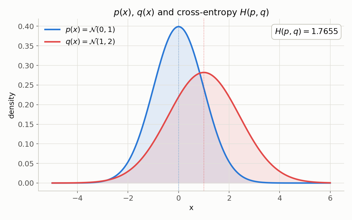
Let \(p = \mathcal{N}(0, 1)\) and \(q = \mathcal{N}(1, 2)\) .

import numpy as np
from scipy.stats import norm

rng = np.random.default_rng(42)

mu1, sigma1_sq = 0.0, 1.0
mu2, sigma2_sq = 1.0, 2.0

# closed form (eq. 1)
H_closed = 0.5 * np.log(2 * np.pi * sigma2_sq) + ((mu1 - mu2) ** 2 + sigma1_sq) / (2 * sigma2_sq)
print(f"closed form: {H_closed:.6f}")

sigma1, sigma2 = np.sqrt(sigma1_sq), np.sqrt(sigma2_sq)
for N in [10_000, 100_000, 1_000_000, 10_000_000]:
    x = rng.normal(mu1, sigma1, size=N)
    H_mc = -np.mean(norm.logpdf(x, loc=mu2, scale=sigma2))
    rel_err = abs(H_mc - H_closed) / abs(H_closed)
    print(f"N={N:>10}: MC={H_mc:.6f}  rel_err={rel_err:.3e}")

Output:

closed form: 1.765512
N=     10000: MC=1.773816  rel_err=4.703e-03
N=    100000: MC=1.769089  rel_err=2.026e-03
N=   1000000: MC=1.765015  rel_err=2.814e-04
N=  10000000: MC=1.765362  rel_err=8.501e-05

At \(N=10^7\) the relative error shrinks to \(8.5\times 10^{-5}\) , converging to the closed-form value \(H(p,q)=1.765512\) from equation (1).

Multivariate (2D) case

Let \(p = \mathcal{N}(\boldsymbol{\mu}_1, \Sigma_1)\) and \(q = \mathcal{N}(\boldsymbol{\mu}_2, \Sigma_2)\) with:

import numpy as np
from scipy.stats import multivariate_normal

rng = np.random.default_rng(42)

mu1 = np.array([0.0, 0.0])
Sigma1 = np.array([[1.0, 0.3], [0.3, 1.0]])
mu2 = np.array([1.0, -1.0])
Sigma2 = np.array([[2.0, 0.5], [0.5, 1.5]])
d = 2

Sigma2_inv = np.linalg.inv(Sigma2)
diff = mu1 - mu2

# closed form (eq. 4)
H_closed = 0.5 * (
    d * np.log(2 * np.pi)
    + np.log(np.linalg.det(Sigma2))
    + np.trace(Sigma2_inv @ Sigma1)
    + diff @ Sigma2_inv @ diff
)
print(f"closed form: {H_closed:.6f}")

p = multivariate_normal(mean=mu1, cov=Sigma1)
q = multivariate_normal(mean=mu2, cov=Sigma2)  # independent (scipy) cross-check
for N in [10_000, 100_000, 1_000_000, 10_000_000]:
    x = p.rvs(size=N, random_state=rng)
    H_mc = -np.mean(q.logpdf(x))
    rel_err = abs(H_mc - H_closed) / abs(H_closed)
    print(f"N={N:>10}: MC={H_mc:.6f}  rel_err={rel_err:.3e}")

Output:

closed form: 3.743678
N=     10000: MC=3.747151  rel_err=9.279e-04
N=    100000: MC=3.739399  rel_err=1.143e-03
N=   1000000: MC=3.743999  rel_err=8.594e-05
N=  10000000: MC=3.743508  rel_err=4.515e-05

Re-running with an independent random seed at \(N=2\times10^6\) gives MC=3.743115 (relative error \(1.50\times10^{-4}\) ), confirming this is not a coincidence tied to one particular random stream. A 3D case (\(\boldsymbol{\mu}_1=[0,1,-1]\) with non-diagonal \(\Sigma_1, \Sigma_2\) ) was also verified: the closed form gives \(H(p,q)=5.040413\) , and Monte Carlo with \(N=10^7\) converges to a relative error of \(1.35\times10^{-5}\) .

Numerical verification of the KL-divergence relation

The relations in equations (5)–(7) were also verified numerically. For the univariate example (\(p=\mathcal{N}(0,1)\) , \(q=\mathcal{N}(1,2)\) ):

Comparing this against a direct evaluation of the standard formula (7) gives an exact match (the only discrepancy is double-precision rounding error, \(< 10^{-15}\) ). For the 2D example, \(H(p,q)-H(p) = 0.952956\) likewise matches the direct evaluation of equation (7) to within \(3.3\times10^{-16}\) . The algebra that cancels the \(d\ln(2\pi)\) terms in the derivation therefore holds numerically as well, not just symbolically.

Visualizing the convergence

The two Gaussians \(p(x)\) and \(q(x)\) along with the value of their cross-entropy (univariate example, \(H(p,q)=1.7655\) ) are shown below.

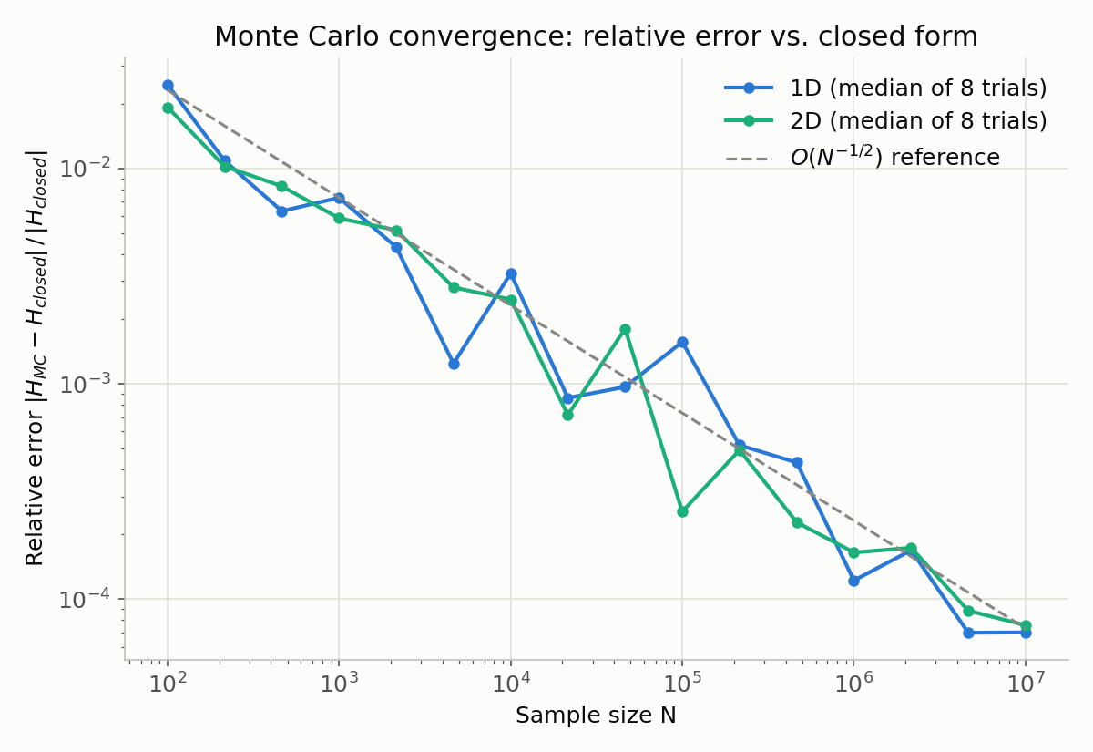
The plot below shows the relative error against sample size \(N\) , from \(10^2\) to \(10^7\) on a log-log scale, for both the univariate and 2D cases (median of 8 trials per \(N\) ). The error decreases roughly along the \(O(N^{-1/2})\) rate typical of Monte Carlo estimation (dashed reference line, slope \(-1/2\) ), dropping below \(10^{-4}\) relative error by \(N=10^7\) .

Summary

• The univariate cross-entropy \(H(p_1,p_2) = \frac{1}{2}\log(2\pi\sigma_2^2) + \frac{(\mu_1-\mu_2)^2+\sigma_1^2}{2\sigma_2^2}\) was generalized to the multivariate closed form \(H(p,q) = \frac{1}{2}[d\ln(2\pi)+\ln|\Sigma_2|+\mathrm{tr}(\Sigma_2^{-1}\Sigma_1)+(\boldsymbol{\mu}_1-\boldsymbol{\mu}_2)^\top\Sigma_2^{-1}(\boldsymbol{\mu}_1-\boldsymbol{\mu}_2)]\) , using the trace trick \(\mathbb{E}[\boldsymbol{x}^\top A\boldsymbol{x}]=\mathrm{tr}(A\,\mathrm{Cov}(\boldsymbol{x}))+\mathbb{E}[\boldsymbol{x}]^\top A\,\mathbb{E}[\boldsymbol{x}]\) .
• Via \(D_{KL}(p\|q) = H(p,q) - H(p)\) , the standard closed-form multivariate Gaussian KL divergence was recovered by simply subtracting the known self-entropy \(H(p)=\frac{1}{2}\ln((2\pi e)^d|\Sigma_1|)\) .
• Loss functions for heteroscedastic regression and VAE reconstruction terms — anywhere continuous output is modeled as a Gaussian — reduce to this cross-entropy form.
• The closed form was cross-checked against Monte Carlo estimation in 1D, 2D, and 3D, converging to relative errors on the order of \(10^{-4}\) –\(10^{-5}\) at \(N=10^7\) , and the decomposition into KL divergence was confirmed to hold numerically as well.

References

• C.M. Bishop, Pattern Recognition and Machine Learning , Springer (2006)