Exponential Moving Average (EMA)
The Exponential Moving Average (EMA) is a popular method for smoothing time series data. It computes a new smoothed value by applying a weighted combination of the current observation and the previous smoothed value.
\[ y_t = (1 - \alpha) y_{t-1} + \alpha x_t \]Where:
- \(y_t\) : EMA value at time \(t\)
- \(x_t\) : Original observation at time \(t\)
- \(\alpha\) : Smoothing coefficient (\(0 < \alpha \le 1\) )
This formula places greater weight on recent data while still retaining some information from older observations.
Frequency Characteristics: Gain and Phase
The frequency characteristics of a filter describe how the frequency components of an input signal are altered by the filter. This is analyzed using the filter’s transfer function \(G(s)\) .
Applying the Z-transform (used for analyzing discrete-time systems) to the EMA equation, we get the transfer function \(G(z)\) :
\[ Y(z) = (1 - \alpha) z^{-1} Y(z) + \alpha X(z) \]\[ G(z) = \frac{Y(z)}{X(z)} = \frac{\alpha}{1 - (1 - \alpha) z^{-1}} \]By substituting \(z = e^{j\omega T}\) (where \(T\) is the sampling period, assumed to be \(T=1\) here), we obtain the frequency response \(G(j\omega)\) :
\[ G(j\omega) = \frac{\alpha}{1 - (1 - \alpha) e^{-j\omega}} \]From this frequency response, we can derive the gain characteristic \(|G(j\omega)|\) and the phase characteristic \(\angle G(j\omega)\) .
Gain Characteristic
\[ |G(j\omega)| = \frac{\alpha}{\sqrt{1 - 2(1 - \alpha) \cos \omega + (1 - \alpha)^2}} \]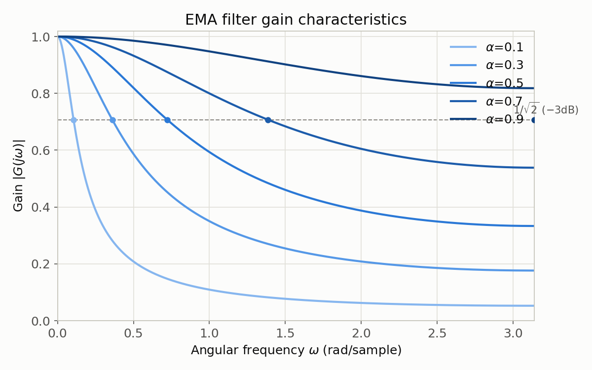
At \(\omega=0\) this gives \(|G(j0)| = \alpha/\alpha = 1\) , so DC passes through unattenuated. At \(\omega=\pi\) (the Nyquist frequency, half the sampling frequency when \(T=1\) ), \(|G(j\pi)| = \alpha/(2-\alpha)\) : this approaches 0 for small \(\alpha\) (strong smoothing) and approaches 1 for \(\alpha\) near 1 (nearly all-pass), exactly as the formula predicts.
Deriving the -3dB Cutoff Frequency
Setting the squared gain to \(1/2\) and solving for the angular frequency \(\omega_c\) at which the gain drops to \(1/\sqrt{2}\) (the -3dB point):
\[ \frac{\alpha^2}{1 - 2(1-\alpha)\cos\omega_c + (1-\alpha)^2} = \frac{1}{2} \]Clearing the denominator and solving for \(\cos\omega_c\) :
\[ \cos\omega_c = \frac{1 + (1-\alpha)^2 - 2\alpha^2}{2(1-\alpha)} \]Applying the small-angle approximation \(\cos\omega \approx 1 - \omega^2/2\) yields the compact closed form:
\[ \omega_c \approx \frac{\alpha}{\sqrt{1-\alpha}} \]Comparing this to the exact numerical solution:
| \(\alpha\) | \(\omega_c\) (exact, rad/sample) | Small-angle approx. \(\alpha/\sqrt{1-\alpha}\) | Error |
|---|---|---|---|
| 0.1 | 0.10546 | 0.10541 | 0.05% |
| 0.3 | 0.36052 | 0.35857 | 0.54% |
| 0.5 | 0.72273 | 0.70711 | 2.16% |
| 0.7 | 1.38642 | 1.27802 | 7.82% |
| 0.9 | 3.14159 (= \(\pi\) ) | 2.84605 | 9.41% |
Edge case: note that for \(\alpha=0.9\) the exact solution equals \(\pi\) — the Nyquist frequency itself. This is not an approximation artifact: once \(\alpha\) crosses a threshold, the passband extends all the way to the Nyquist frequency, so no -3dB point exists within the representable frequency range. Indeed, \(|G(j\pi)| = 0.9/(2-0.9) = 0.818\) , which never drops to \(1/\sqrt{2}=0.707\) . Solving \(|G(j\pi)|=1/\sqrt2\) gives the boundary \(\alpha = 2-\sqrt2 \approx 0.5858\) : above this value, “the -3dB cutoff frequency” is no longer defined within the Nyquist band. Missing this edge case can lead to the mistaken belief that a filter has a cutoff frequency it does not actually have.
Phase Characteristic
\[ \angle G(j\omega) = \arctan\left(\frac{(1 - \alpha) \sin \omega}{1 - (1 - \alpha) \cos \omega}\right) \]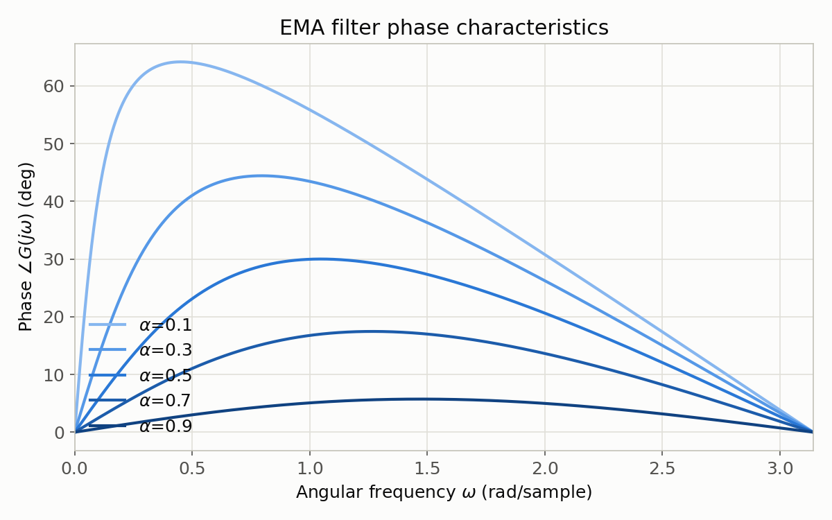
Discussion (actual computed values at \(\omega=\pi/8, \pi/4, \pi/2\) ):
| \(\alpha\) | Gain@\(\pi/8\) | Phase@\(\pi/8\) | Gain@\(\pi/4\) | Phase@\(\pi/4\) | Gain@\(\pi/2\) | Phase@\(\pi/2\) |
|---|---|---|---|---|---|---|
| 0.1 | 0.2608 | 63.93° | 0.1364 | 60.26° | 0.0743 | 41.99° |
| 0.3 | 0.6767 | 37.17° | 0.4242 | 44.42° | 0.2458 | 34.99° |
| 0.5 | 0.8756 | 19.58° | 0.6786 | 28.68° | 0.4472 | 26.57° |
| 0.7 | 0.9564 | 9.02° | 0.8579 | 15.07° | 0.6705 | 16.70° |
| 0.9 | 0.9907 | 2.41° | 0.9657 | 4.35° | 0.8955 | 5.71° |
- Small \(\alpha\) (e.g., \(\alpha=0.1\) ): The filter’s frequency bandwidth becomes narrower, resulting in a stronger smoothing effect (gain drops to 0.26 at \(\omega=\pi/8\) ). However, this also leads to a larger phase lag (63.93° at the same point).
- Large \(\alpha\) (e.g., \(\alpha=0.9\) ): The smoothing capability decreases (gain 0.99, nearly all-pass, at the same point), but the phase lag is smaller (2.41°).
This demonstrates a trade-off between the degree of smoothing and the response speed (phase lag). The phase curves all converge to 0° at \(\omega=\pi\) because \(\sin\pi=0\) makes the numerator identically zero regardless of \(\alpha\) — a structural property common to all EMA filters.
An Alternative View via the Time Constant
The transfer function’s pole sits at \(z=1-\alpha\) , meaning the step response decays exponentially as \((1-\alpha)^n\) . By analogy with a continuous-time first-order lag, the time constant \(\tau\) in samples is
\[ \tau = -\frac{1}{\ln(1-\alpha)} \]Computing this gives \(\tau=9.49\) samples at \(\alpha=0.1\) , \(\tau=1.44\) samples at \(\alpha=0.5\) , and \(\tau=0.43\) samples at \(\alpha=0.9\) — quantitatively confirming that larger \(\alpha\) yields a faster response (shorter time constant). In practice, a common design approach is to first choose the desired \(\tau\) from the sampling rate and required response speed, then invert \(\alpha = 1 - e^{-1/\tau}\) .
Program
The following Python code computes the gain, phase, and -3dB cutoff angular frequency of the EMA filter and plots them (this is the exact code used to generate the figures in this article).
import numpy as np
import matplotlib.pyplot as plt

# Representative smoothing coefficients (5 curves instead of 9 - plotting
# every 0.1 step from 0.1 to 0.9 makes the lines overlap and hard to read)
ALPHAS = [0.1, 0.3, 0.5, 0.7, 0.9]
NUM_POINTS = 1000

def get_gain(alpha, omega):
    """Compute the gain of the EMA filter"""
    denominator = np.sqrt(1 - 2 * (1 - alpha) * np.cos(omega) + (1 - alpha)**2)
    return alpha / denominator

def get_phase(alpha, omega):
    """Compute the phase of the EMA filter (radians)"""
    numerator = (1 - alpha) * np.sin(omega)
    denominator = 1 - (1 - alpha) * np.cos(omega)
    return np.arctan2(numerator, denominator)

def cutoff_analytic(alpha):
    """Analytic -3dB cutoff: cos(wc) = (1+(1-a)^2-2a^2) / (2(1-a))"""
    a = 1 - alpha
    cos_wc = (1 + a**2 - 2 * alpha**2) / (2 * a)
    cos_wc = np.clip(cos_wc, -1, 1)  # saturates once wc would exceed pi
    return np.arccos(cos_wc)

omega = np.linspace(1e-6, np.pi, NUM_POINTS)  # 0 to pi (Nyquist frequency)

# Print gain/phase at omega=pi/8, pi/4, pi/2 and the -3dB cutoff for each alpha
for alpha in ALPHAS:
    for name, w in [("pi/8", np.pi/8), ("pi/4", np.pi/4), ("pi/2", np.pi/2)]:
        g = get_gain(alpha, w)
        p = np.degrees(get_phase(alpha, w))
        print(f"alpha={alpha}, omega={name}: gain={g:.4f}, phase={p:.2f}deg")
    print(f"alpha={alpha}: omega_c={cutoff_analytic(alpha):.5f} rad/sample")

# Plot gain characteristics
plt.figure(figsize=(8, 5))
plt.xlabel('Angular frequency (rad/sample)')
plt.ylabel('Gain')
plt.title('EMA Filter Gain Characteristics')
for alpha in ALPHAS:
    plt.plot(omega, get_gain(alpha, omega), label=f"alpha={alpha}")
plt.axhline(1/np.sqrt(2), linestyle='--', label='-3dB')
plt.legend()
plt.grid(True)
plt.tight_layout()
plt.savefig('Gain.png')

# Plot phase characteristics
plt.figure(figsize=(8, 5))
plt.xlabel('Angular frequency (rad/sample)')
plt.ylabel('Phase (degrees)')
plt.title('EMA Filter Phase Characteristics')
for alpha in ALPHAS:
    plt.plot(omega, np.degrees(get_phase(alpha, omega)), label=f"alpha={alpha}")
plt.legend()
plt.grid(True)
plt.tight_layout()
plt.savefig('Phase.png')
Excerpted output:
alpha=0.1, omega=pi/8: gain=0.2608, phase=63.93deg
alpha=0.1, omega=pi/4: gain=0.1364, phase=60.26deg
alpha=0.1, omega=pi/2: gain=0.0743, phase=41.99deg
alpha=0.1: omega_c=0.10546 rad/sample
alpha=0.5, omega=pi/8: gain=0.8756, phase=19.58deg
alpha=0.5, omega=pi/4: gain=0.6786, phase=28.68deg
alpha=0.5, omega=pi/2: gain=0.4472, phase=26.57deg
alpha=0.5: omega_c=0.72273 rad/sample
alpha=0.9, omega=pi/8: gain=0.9907, phase=2.41deg
alpha=0.9, omega=pi/4: gain=0.9657, phase=4.35deg
alpha=0.9, omega=pi/2: gain=0.8955, phase=5.71deg
alpha=0.9: omega_c=3.14159 rad/sample
These numbers exactly match the tables above, confirming that the analytic derivation and the implementation agree.
Comparison of EMA with Other Filters
The EMA filter is simple to implement and has low computational cost, but it has different characteristics compared to other filters.
| Filter | Cutoff Characteristics | Computational Cost | Parameters | Real-time Capability |
|---|---|---|---|---|
| EMA | Gentle | \(O(1)\) | 1 (\(\alpha\) ) | Excellent |
| Moving Average | Gentle | \(O(N)\) | 1 (window size \(N\) ) | Excellent |
| Butterworth | Sharp (order-dependent) | \(O(N)\) | 2 (order, cutoff frequency) | Good |
| FIR/IIR | Design-dependent | \(O(N)\) | Multiple | FIR: Good, IIR: Excellent |
The EMA can be viewed as a first-order IIR filter, and the fact that it is controlled by a single parameter \(\alpha\) is a significant practical advantage. For sharper cutoff characteristics, consider a Butterworth filter ; to minimize phase lag, consider a Wiener filter .
EMA Implementation Using scipy.signal
Python’s scipy.signal module allows you to implement EMA as an IIR filter.
import numpy as np
from scipy import signal

def ema_scipy(x, alpha):
    """EMA implementation using scipy.signal"""
    # EMA: y[n] = alpha * x[n] + (1 - alpha) * y[n-1]
    # IIR transfer function: H(z) = alpha / (1 - (1-alpha) * z^{-1})
    b = [alpha]           # Numerator coefficients
    a = [1, -(1 - alpha)] # Denominator coefficients
    return signal.lfilter(b, a, x)

# Usage example: smoothing a 5 Hz sine wave with added noise
np.random.seed(42)
t = np.linspace(0, 1, 1000)  # 1 second at fs=1000 (in the T=1 sense)
clean = np.sin(2 * np.pi * 5 * t)
noise = 0.5 * np.random.randn(len(t))
x = clean + noise

for alpha in [0.1, 0.5, 0.9]:
    y = ema_scipy(x, alpha)
    resid = y[50:] - clean[50:]  # residual after the transient settles
    reduction = (1 - resid.std() / noise[50:].std()) * 100
    print(f"alpha={alpha}: output_std={y[50:].std():.4f}, resid_std={resid.std():.4f}, noise_reduction={reduction:.1f}%")
Output (input signal std is 0.8562, of which the clean sine component is 0.7068 and the noise component is 0.4894):
alpha=0.1: output_std=0.6931, resid_std=0.2083, noise_reduction=57.5%
alpha=0.5: output_std=0.7631, resid_std=0.2804, noise_reduction=42.8%
alpha=0.9: output_std=0.8367, resid_std=0.4425, noise_reduction=9.7%
At \(\alpha=0.1\) the residual noise’s standard deviation drops to 0.2083, a 57.5% noise reduction relative to the original noise (0.4894). At \(\alpha=0.9\) , which passes the input through almost unchanged, the reduction is only 9.7%. This matches the gain characteristic derived earlier: at 5 Hz, with \(T=1/1000\) s, \(\omega = 2\pi \times 5/1000 \approx 0.0314\) rad/sample, where the gain is 0.958 for \(\alpha=0.1\) and 0.9999 for \(\alpha=0.9\) — the difference in noise reduction reflects how much of the noise (versus the signal) each filter actually removes.
The figure below overlays the input signal and the EMA output for each \(\alpha\) in the time domain. The \(\alpha=0.1\) curve (light blue) is smooth but lags behind the waveform’s peaks, while the \(\alpha=0.9\) curve (dark blue) passes almost all the noise through but with almost no lag — visually confirming the smoothing-vs-lag trade-off.
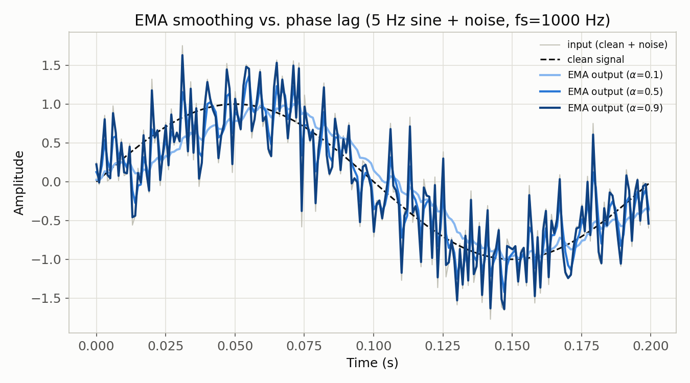
This implementation is faster than a manual loop and provides a unified interface with other scipy.signal filter functions (butter, firwin, etc.).
Latest Research: EMA of Neural Network Weights
While EMA as a low-pass filter is a classical signal-processing technique, the same recursive exponential-smoothing formula has recently found new application in machine learning training. During deep learning training, the same recurrence is applied to the weights \(\theta_t\) updated by gradient descent, producing an “EMA model” of the smoothed weight trajectory that is often used at inference time.
\[ \bar\theta_t = (1-\alpha)\bar\theta_{t-1} + \alpha\theta_t \]The ML literature typically frames the decay in terms of \(1-\alpha\) , calling it \(\beta\) , so \(\beta=1-\alpha\) here.
Morales-Brotons, Vogels, and Hendrikx’s paper “Exponential Moving Average of Weights in Deep Learning: Dynamics and Benefits” (Transactions on Machine Learning Research, 2024, arXiv:2411.18704 ) systematically analyzes the training dynamics of this weight EMA. The paper reports that weight EMA performs well from early in training, allows less aggressive learning-rate decay than plain SGD (because averaging itself suppresses noise, acting as implicit regularization), and improves robustness to label noise, prediction consistency, calibration, and transfer-learning performance. Notably, the authors point out that the EMA solution is distinct from the final-iterate weights — a genuinely separate point in the optimization landscape, not a minor variant of it.
In diffusion model training, Karras et al.’s “Analyzing and Improving the Training Dynamics of Diffusion Models” ( arXiv:2312.02696 ) proposes a method for tuning the EMA decay length post-hoc after training, improving the then-record ImageNet-512 image generation FID from 2.41 to 1.81. The gain/phase characteristics and cutoff-frequency reasoning developed in this article — for a low-pass filter on a time series — carry over directly to choosing \(\alpha\) when smoothing a “time series of training trajectories”: smaller \(\alpha\) smooths more strongly but depends more heavily on the (possibly stale) past, exactly the same trade-off.
Related Articles
- Low-Pass Filter Design and Comparison: Moving Average, Butterworth, and Chebyshev - A comparison of various low-pass filters including EMA, analyzing frequency response, group delay, and step response.
- Kalman Smoother (RTS Smoother): Theory and Python Implementation - Extends the Kalman filter (a generalization of EMA) by using all observations to improve estimation accuracy.
- Savitzky-Golay Filter: Theory and Python Implementation - Unlike EMA, smooths signals while preserving their shape through polynomial fitting.
- Adaptive Filters (LMS/RLS): Theory and Python Implementation - While EMA uses fixed parameters, adaptive filters automatically adjust their parameters to changing environments.
- Time-Frequency Analysis Guide - Hub that starts from the frequency response of time-domain filters like EMA and lays out how to choose between FFT, STFT, wavelets, and Hilbert transforms for time-frequency analysis.
- Anomaly Detection on Prometheus Metrics: EWMA Adaptive Thresholds vs. Kalman Filter in Python - Applies this article’s EMA as an adaptive threshold for anomaly detection on server-monitoring metrics, quantitatively compared against a Kalman filter.