In deep learning models, sampling from a probability distribution is typically a non-differentiable operation. This makes it impossible to use backpropagation to compute gradients and update model parameters.
To address this issue, D. P. Kingma and M. Welling introduced the Reparameterization Trick in their Variational Autoencoder (VAE) paper.
Principle
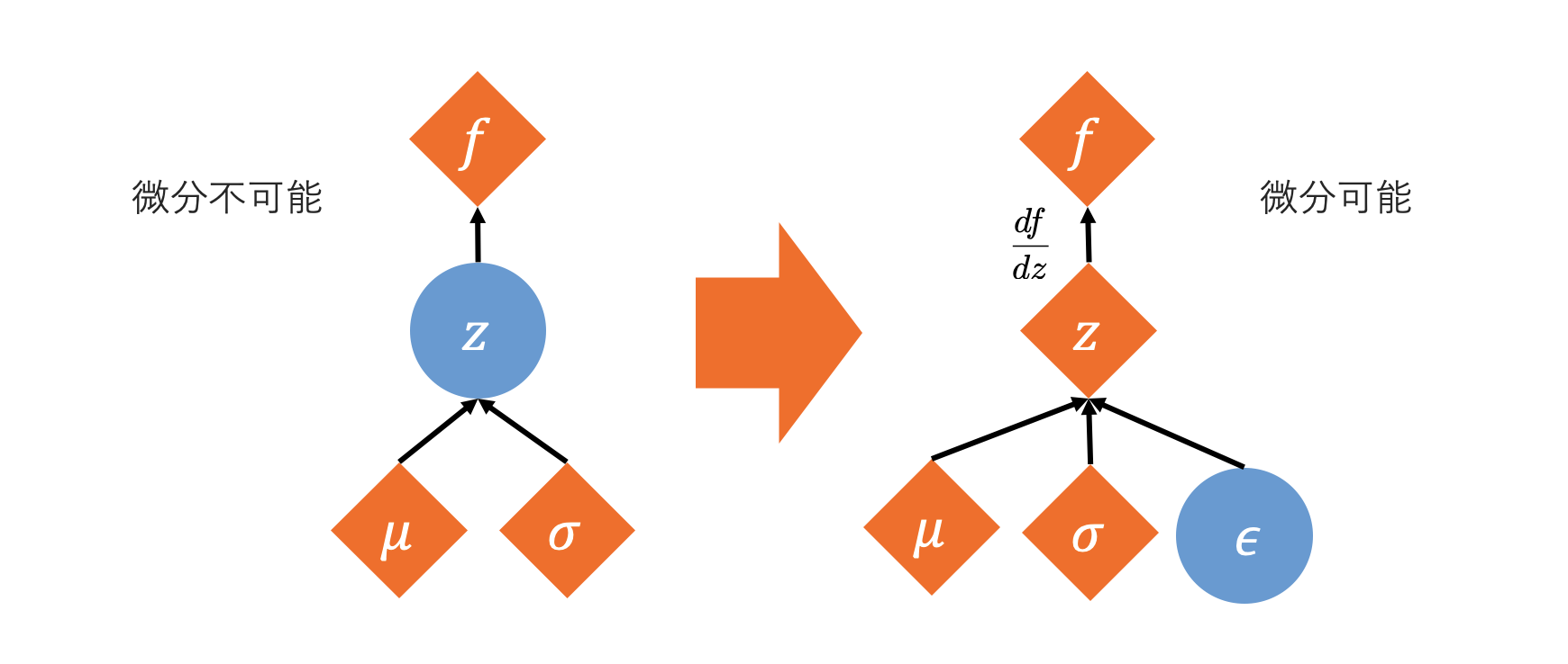
The Reparameterization Trick makes the sampling process differentiable by separating the sampling operation into two parts: random noise independent of the parameters and a deterministic transformation dependent on the parameters.
For example, consider sampling a random variable \(z\) from a normal distribution \(\mathcal{N}(\mu, \sigma^2)\) with mean \(\mu\) and variance \(\sigma^2\) :
\[ z \sim \mathcal{N}(\mu, \sigma^2) \]This sampling operation is non-differentiable. However, by using random noise \(\epsilon\) sampled from a standard normal distribution \(\mathcal{N}(0, 1)\) , \(z\) can be expressed as:
\[ z = \mu + \sigma \odot \epsilon \]\[ \text{where } \epsilon \sim \mathcal{N}(0, 1) \](\(\odot\) denotes element-wise multiplication. In the multi-dimensional case, \(\sigma\) corresponds to the vector of standard deviations or the square root of the covariance matrix.)
This transformation makes \(z\) a deterministic function with respect to \(\mu\) and \(\sigma\) , allowing \(\mu\) and \(\sigma\) (which are typically outputs of a neural network) to be differentiable. The randomness is encapsulated in \(\epsilon\) , and gradients can be backpropagated through \(\mu\) and \(\sigma\) .
Why Reparameterization Is Necessary: The Gradient-of-Expectation Problem
In VAE training, we use samples \(z\) drawn from a distribution \(q_\phi(z)\) that depends on the encoder parameters \(\phi\) to maximize an objective (part of the ELBO)
\[ L(\phi) = \mathbb{E}_{z \sim q_\phi(z)}[f(z)] = \int f(z)\, q_\phi(z)\, dz \]where \(f\) is, for example, the decoder’s log-likelihood. To update \(\phi\) with gradient methods we need \(\nabla_\phi L(\phi)\) , but this is less trivial than it looks: because \(q_\phi\) itself depends on \(\phi\) ,
\[ \nabla_\phi \mathbb{E}_{z \sim q_\phi}[f(z)] \neq \mathbb{E}_{z \sim q_\phi}[\nabla_\phi f(z)] \]The right-hand side differentiates \(f\) with respect to \(\phi\) while holding \(z\) fixed, but the distribution of \(z\) itself moves with \(\phi\) , so this expression discards exactly the information we need. Formally exchanging the gradient and the integral gives
\[ \nabla_\phi L(\phi) = \int f(z)\, \nabla_\phi q_\phi(z)\, dz \tag{1} \]so the integrand is \(f(z)\nabla_\phi q_\phi(z)\) , not \(\nabla_\phi f(z)\) . Worse, \(\nabla_\phi q_\phi(z)\) is not itself a probability density (it need not integrate to 1), so the natural Monte Carlo recipe — “sample from \(q_\phi\) and average” — does not directly apply to Eq. (1). This is the crux of the problem: how do we obtain an unbiased, low-variance Monte Carlo estimator for the gradient of an expectation whose sampling distribution depends on the parameter we’re differentiating with respect to?
The reparameterization trick sidesteps this. If \(z\) can be written as a composition of a base distribution \(p(\epsilon)\) that does not depend on \(\phi\) , and a deterministic transformation \(g_\phi\) that does,
\[ z = g_\phi(\epsilon), \qquad \epsilon \sim p(\epsilon) \](for a Gaussian, \(g_\phi(\epsilon) = \mu + \sigma \odot \epsilon\) ), then the objective becomes
\[ L(\phi) = \mathbb{E}_{\epsilon \sim p(\epsilon)}[f(g_\phi(\epsilon))] = \int f(g_\phi(\epsilon))\, p(\epsilon)\, d\epsilon \]Now the expectation is taken over a fixed distribution \(p(\epsilon)\) that does not depend on \(\phi\) , so under mild regularity conditions (e.g. \(f \circ g_\phi\) dominated by a \(\phi\) -integrable function) we can freely exchange gradient and integral:
\[ \nabla_\phi L(\phi) = \int \nabla_\phi f(g_\phi(\epsilon))\, p(\epsilon)\, d\epsilon = \mathbb{E}_{\epsilon \sim p(\epsilon)}[\nabla_\phi f(g_\phi(\epsilon))] \tag{2} \]Equation (2) can be estimated unbiasedly by drawing one or more samples \(\epsilon \sim p(\epsilon)\) and differentiating \(f(g_\phi(\epsilon))\) with respect to \(\phi\) using ordinary backpropagation (the chain rule). Because the source of randomness \(\epsilon\) has a fixed distribution, we no longer need to worry about the order of “sampling” and “differentiating” — that is the essence of the reparameterization trick.
Comparison with REINFORCE (the Score-Function Estimator)
There is another way to turn Eq. (1) into a Monte Carlo estimator directly: the log-derivative trick. The gradient of a density can be written as
\[ \nabla_\phi q_\phi(z) = q_\phi(z)\, \nabla_\phi \log q_\phi(z) \](multiply both sides of \(\nabla_\phi \log q_\phi(z) = \nabla_\phi q_\phi(z) / q_\phi(z)\) by \(q_\phi(z)\) ). Substituting into Eq. (1) gives
\[ \nabla_\phi L(\phi) = \int f(z)\, q_\phi(z)\, \nabla_\phi \log q_\phi(z)\, dz = \mathbb{E}_{z \sim q_\phi}\left[f(z)\, \nabla_\phi \log q_\phi(z)\right] \tag{3} \]Now the expectation is taken under \(q_\phi(z)\) (which does depend on \(\phi\) ), but the integrand \(f(z)\nabla_\phi \log q_\phi(z)\) is an ordinary function, so we can simply sample \(z \sim q_\phi\) in the usual way and average to get an unbiased estimator. This is the REINFORCE estimator (also called the score-function estimator), and its derivation is exactly the log-derivative trick used in the policy gradient theorem for policy gradient methods in reinforcement learning. Its key advantage is that \(z\) need not be a differentiable function of \(\phi\) — it works even when \(z\) is discrete. The reparameterization trick, in contrast, requires the existence of a differentiable map \(z = g_\phi(\epsilon)\) , so in principle it only applies to continuous variables.
The trade-off is that REINFORCE is well known to have much higher variance. To make this concrete, consider \(q_\phi = \mathcal{N}(\mu, \sigma^2)\) (with \(\phi = \mu\) and \(\sigma\) fixed) and \(f(z) = z^2\) , and derive both estimators explicitly.
- REINFORCE estimator: since \(\log q_\phi(z) = -\frac{1}{2}\log(2\pi\sigma^2) - \frac{(z-\mu)^2}{2\sigma^2}\) , we get \(\nabla_\mu \log q_\phi(z) = (z-\mu)/\sigma^2\) , so the per-sample estimator from Eq. (3) is
- Reparameterization estimator: with \(z = \mu + \sigma\epsilon\) and \(f(z)=z^2\) , \(\nabla_\mu f(z) = 2z \cdot \frac{\partial z}{\partial \mu} = 2z\) , so
The true gradient is \(\nabla_\mu \mathbb{E}[z^2] = 2\mu\) , since \(\mathbb{E}[z^2] = \mu^2+\sigma^2\) . Writing \(u = z-\mu \sim \mathcal{N}(0,\sigma^2)\) and using the central moments of a Gaussian (\(\mathbb{E}[u]=\mathbb{E}[u^3]=\mathbb{E}[u^5]=0\) , \(\mathbb{E}[u^2]=\sigma^2\) , \(\mathbb{E}[u^4]=3\sigma^4\) , \(\mathbb{E}[u^6]=15\sigma^6\) ), we can compute both variances analytically:
\[ \mathrm{Var}(\hat{g}_{\text{reparam}}) = 4\sigma^2 \] \[ \mathrm{Var}(\hat{g}_{\text{REINFORCE}}) = 15\sigma^2 + 14\mu^2 + \frac{\mu^4}{\sigma^2} \](the second is obtained by expanding \(\hat g_{\text{REINFORCE}}=(u^3+2\mu u^2+\mu^2 u)/\sigma^2\) , using the fact that odd central moments vanish to compute \(\mathbb{E}[\hat g_{\text{REINFORCE}}^2]\) , then subtracting \((2\mu)^2\) ). Substituting \(\mu=1,\sigma=1\) gives an exact variance ratio of
\[ \frac{\mathrm{Var}(\hat{g}_{\text{REINFORCE}})}{\mathrm{Var}(\hat{g}_{\text{reparam}})} = \frac{15+14+1}{4} = \frac{30}{4} = 7.5 \]We verified this theoretical prediction with an actual Python Monte Carlo experiment.
import numpy as np

rng = np.random.default_rng(42)
mu, sigma = 1.0, 1.0
n = 5_000_000

z = rng.normal(mu, sigma, size=n)
g_reinforce = z**2 * (z - mu) / sigma**2
g_reparam = 2 * z

print("Var(REINFORCE):", g_reinforce.var())   # theory: 30
print("Var(reparam):  ", g_reparam.var())     # theory: 4
print("ratio:", g_reinforce.var() / g_reparam.var())  # theory: 7.5
The result was Var(REINFORCE) = 30.037, Var(reparam) = 3.998, ratio 7.513 — an excellent match with the theoretical values (30, 4, 7.5). With \(\mu=0\)
the theoretical ratio drops to \(15/4=3.75\)
; the empirical result was Var(REINFORCE)=15.023, Var(reparam)=3.998, ratio 3.758, again matching theory (note that REINFORCE’s variance does not vanish at \(\mu=0\)
).
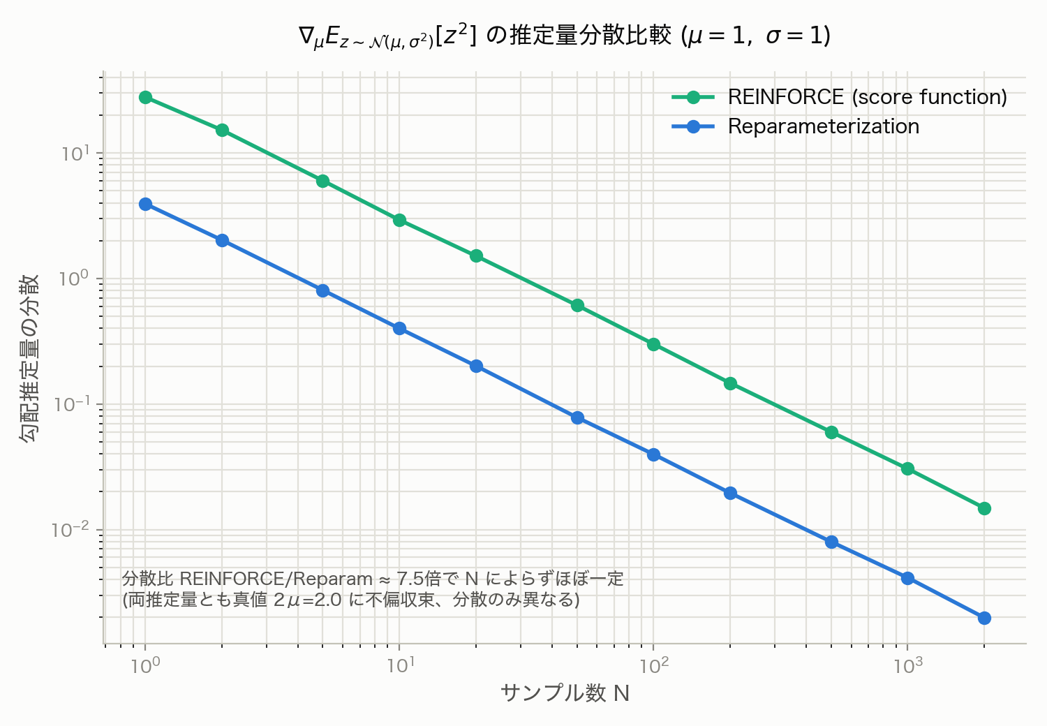
We also measured the variance of the sample-mean estimator as the number of samples \(N\) grows (\(\mu=1,\sigma=1\) , 20,000 Monte Carlo trials per setting):
| \(N\) | REINFORCE var. | Reparam var. | Ratio |
|---|---|---|---|
| 1 | 31.640 | 4.005 | 7.90 |
| 10 | 3.043 | 0.397 | 7.66 |
| 100 | 0.304 | 0.0395 | 7.69 |
| 1000 | 0.0303 | 0.00398 | 7.63 |
Both estimators’ variance shrinks as \(1/N\) (a consequence of the central limit theorem), and both converge unbiasedly to the true gradient \(2\mu=2.0\) , but REINFORCE remains roughly 7.5x noisier at every sample size — the ratio is essentially constant. Sweeping \(N\) from 1 to 2000 on a log scale confirms this: the two curves decay in parallel.
This variance gap tends to worsen with dimensionality \(d\) (REINFORCE’s variance generally scales unfavorably with the number of dimensions), which is the practical reason the reparameterization trick is the default choice for training deep generative models whenever it is applicable. Conversely, when \(z\) is discrete and cannot be reparameterized, one must fall back on REINFORCE combined with variance-reduction techniques such as baseline subtraction (the same idea used by the advantage function in Actor-Critic ).
Extending to Multivariate and Non-Gaussian Distributions
Multivariate Gaussian with Diagonal Covariance
When the encoder outputs \(\mu, \sigma \in \mathbb{R}^d\) for an independent, diagonal-covariance Gaussian \(\Sigma = \mathrm{diag}(\sigma_1^2,\dots,\sigma_d^2)\) , the formula \(z = \mu + \sigma \odot \epsilon\) already shown above (with \(\epsilon \sim \mathcal{N}(0, I_d)\) and \(\odot\) elementwise product) is directly the multivariate reparameterization. Since the dimensions are independent, the fact that this transformation produces \(z\) with covariance \(\Sigma\) follows trivially from the one-dimensional case applied per coordinate.
Full Covariance via Cholesky Decomposition
For a general covariance matrix \(\Sigma\) (symmetric positive semi-definite) with correlated dimensions, we use the Cholesky decomposition \(\Sigma = LL^\top\) (\(L\) lower-triangular). With \(\epsilon \sim \mathcal{N}(0, I_d)\) , setting
\[ z = \mu + L\epsilon \]gives a random variable with mean \(\mu\) and covariance \(\mathrm{Cov}(z) = L\,\mathrm{Cov}(\epsilon)\,L^\top = L I_d L^\top = LL^\top = \Sigma\) (using \(\mathrm{Cov}(Az)=A\,\mathrm{Cov}(z)\,A^\top\) for linear transforms). As long as \(L\) is a differentiable function of \(\phi\) , gradients propagate through it exactly as in the diagonal case. We verified this procedure numerically with a random 3-dimensional SPD (symmetric positive-definite) matrix \(\Sigma\) and mean vector \(\mu\) .
import numpy as np

rng = np.random.default_rng(1)
d = 3
A = rng.normal(size=(d, d))
Sigma = A @ A.T + d * np.eye(d)   # random SPD matrix
mu = np.array([1.0, -2.0, 0.5])

L = np.linalg.cholesky(Sigma)
eps = rng.normal(size=(500_000, d))
Z = mu + eps @ L.T

print("sample mean:", Z.mean(axis=0))
print("sample cov:\n", np.cov(Z.T))
With 500,000 samples, the resulting sample mean was [1.0014, -2.0034, 0.5067] (maximum absolute error 0.0067 vs. the target [1.0, -2.0, 0.5]), and the sample covariance matched the target \(\Sigma\)
with a maximum absolute error of 0.0130 — consistent with theory up to Monte Carlo sampling error at this sample size.
Why Discrete Variables Resist Simple Reparameterization, and Gumbel-Softmax
The reparameterization trick does not apply directly to discrete (categorical) variables. Sampling from a categorical distribution with probabilities \(\pi_1,\dots,\pi_K\) (dependent on \(\phi\) ) — whether by thresholding a uniform variable \(u \sim U(0,1)\) against the CDF, or via the Gumbel-Max trick described below — always implements the map “base noise \(\to\) output” as a step function (piecewise constant). A step function has zero gradient almost everywhere, so even though the output is a deterministic function of the noise, moving \(\phi\) only ever changes the output discontinuously; \(\nabla_\phi f(g_\phi(\epsilon))\) in Eq. (2) carries no useful gradient signal. This is precisely why naive reparameterization fails for discrete variables.
Two related techniques address this: the Gumbel-Max trick and Gumbel-Softmax (equivalently, the Concrete distribution). Gumbel-Max reparameterizes categorical sampling exactly (i.e. as an equality in distribution):
\[ z = \arg\max_k \left(\log \pi_k + g_k\right), \qquad g_k \overset{\text{i.i.d.}}{\sim} \mathrm{Gumbel}(0,1) \](with \(g_k = -\log(-\log u_k)\) , \(u_k \sim U(0,1)\) ). The randomness is now confined to \(g_k\) , which does not depend on \(\phi\) , but \(\arg\max\) itself is non-differentiable, so gradients still cannot flow. Gumbel-Softmax relaxes the \(\arg\max\) into a temperature-controlled softmax:
\[ \tilde{z}_k = \frac{\exp\left((\log \pi_k + g_k)/\tau\right)}{\sum_{j=1}^K \exp\left((\log \pi_j + g_j)/\tau\right)} \]As \(\tau \to 0\) , \(\tilde z\) converges in probability to the one-hot Gumbel-Max sample; larger \(\tau\) spreads probability mass across categories into a “softer” sample. We verified this temperature dependence numerically for a 4-category distribution with \(\pi=(0.5,0.3,0.15,0.05)\) .
import numpy as np

rng = np.random.default_rng(7)
pi = np.array([0.5, 0.3, 0.15, 0.05])
logits = np.log(pi)
n = 200_000

g = -np.log(-np.log(rng.uniform(size=(n, 4))))
y = logits + g

# Gumbel-Max: empirical category frequencies
onehot = np.eye(4)[y.argmax(axis=1)]
print("Gumbel-Max empirical frequencies:", onehot.mean(axis=0))

for tau in [0.1, 1.0]:
    soft = np.exp(y / tau)
    soft /= soft.sum(axis=1, keepdims=True)
    print(f"tau={tau}: mean of max component = {soft.max(axis=1).mean():.4f}")
The empirical Gumbel-Max category frequencies were [0.5006, 0.3005, 0.1494, 0.0495], closely matching the target \(\pi=(0.5,0.3,0.15,0.05)\)
(numerical confirmation that the two are exactly equal in distribution). For the temperature dependence, at \(\tau=0.1\)
(low temperature) the mean of the largest softmax component was 0.9554, close to 1 (i.e. nearly one-hot / discrete), whereas at \(\tau=1.0\)
(high temperature) it was only 0.6376, showing probability mass smeared across categories. Lower temperature approximates the discrete distribution more closely, but as \(\tau\to0\)
the variance of \(\nabla_\phi \tilde z\)
diverges, destabilizing gradient estimates — a trade-off practitioners handle by annealing \(\tau\)
during training or combining it with a straight-through estimator.
Practical Considerations
Why Variance Is Parameterized via Log-Variance
VAE implementations typically have the encoder network output the log-variance \(\log\sigma^2\) (or \(\log\sigma\) ) rather than \(\sigma\) or \(\sigma^2\) directly, and recover \(\sigma = \exp(0.5 \log\sigma^2)\) . There are three main reasons.
- Unconstrained optimization: the constraint \(\sigma^2>0\) is converted into the unconstrained parameterization \(\log\sigma^2 \in \mathbb{R}\) . Neural network output layers are naturally unconstrained, so this avoids the need for constrained optimization or extra non-negativity clamps (e.g. ReLU or softplus).
- Numerical stability of gradients: parameterizing \(\sigma\) directly tends to produce unstable gradients and unstable \(\log \sigma^2\) terms (needed for the KL divergence) as \(\sigma\to 0\) . Treating \(\log\sigma^2\) as the free variable turns \(\sigma^2 \to 0\) into the smooth limit \(\log\sigma^2 \to -\infty\) , which is far less prone to exploding or vanishing gradients.
- Guaranteed positivity: \(\sigma = \exp(0.5\log\sigma^2)\) is positive for any real input, so even large parameter updates early in training can never make \(\sigma\) negative or complex.
Closed-Form KL Divergence
The VAE loss includes the KL divergence \(D_{KL}(q_\phi\|p)\) between the posterior \(q_\phi(z|x)=\mathcal{N}(\mu,\mathrm{diag}(\sigma^2))\) and the prior \(p(z)=\mathcal{N}(0,I)\) . When the prior is a standard normal, this KL term has a closed form that requires no numerical integration. In one dimension,
\[ D_{KL}(q\|p) = \mathbb{E}_q\left[\log q(z) - \log p(z)\right] \] \[ \log q(z) = -\frac{1}{2}\log(2\pi\sigma^2) - \frac{(z-\mu)^2}{2\sigma^2}, \qquad \log p(z) = -\frac{1}{2}\log(2\pi) - \frac{z^2}{2} \]so
\[ \log q(z) - \log p(z) = -\frac{1}{2}\log\sigma^2 - \frac{(z-\mu)^2}{2\sigma^2} + \frac{z^2}{2} \]Taking the expectation \(\mathbb{E}_q[\cdot]\) : since \(\mathbb{E}_q[(z-\mu)^2]=\sigma^2\) , the second term becomes \(-\frac12\) ; using \(\mathbb{E}_q[z^2] = \mu^2+\sigma^2\) (from \(\mathrm{Var}(z)=\mathbb{E}[z^2]-\mathbb{E}[z]^2\) ) for the third term gives
\[ D_{KL}(q\|p) = \frac{1}{2}\left(\mu^2+\sigma^2-\log\sigma^2-1\right) \]For a \(d\) -dimensional diagonal-covariance posterior, the dimensions are independent so the KL divergence is additive:
\[ D_{KL}(q_\phi\|p) = \frac{1}{2}\sum_{j=1}^{d}\left(\mu_j^2+\sigma_j^2-\log\sigma_j^2-1\right) \tag{4} \]which is exactly the formula seen throughout VAE implementations. We checked this closed form against Monte Carlo integration.
import numpy as np

rng = np.random.default_rng(1)
mu = np.array([0.5, -1.2, 2.0])
log_var = np.array([-0.3, 0.8, 0.1])

# closed form (Eq. 4)
kl_analytic = 0.5 * np.sum(np.exp(log_var) + mu**2 - 1.0 - log_var)

# Monte Carlo integration
sigma = np.exp(0.5 * log_var)
n = 2_000_000
z = mu + sigma * rng.normal(size=(n, 3))
log_q = -0.5*np.sum(np.log(2*np.pi*sigma**2) + ((z-mu)/sigma)**2, axis=1)
log_p = -0.5*np.sum(np.log(2*np.pi) + z**2, axis=1)
kl_mc = np.mean(log_q - log_p)

print(f"analytic: {kl_analytic:.6f}")
print(f"Monte Carlo (n=2e6): {kl_mc:.6f}")
The result was 3.080765 for the closed form and 3.081169 for the Monte Carlo estimate (2,000,000 samples), a difference of only 0.000404 — strong numerical confirmation of Eq. (4). This closed form is what allows the reconstruction term (estimated via reparameterization) and the KL term (computed exactly) to be combined into the standard VAE loss without any additional sampling.
Sampling Using the Reparameterization Trick in PyTorch
PyTorch’s torch.distributions module provides distributions that support the reparameterization trick. Distribution objects such as the Normal class support reparameterized sampling through the rsample() method.
import torch
from torch.distributions import Normal

# Mean and standard deviation obtained as neural network outputs
# As an example, consider a normal distribution with mu=0, sigma=1
mu = torch.tensor(0.0, requires_grad=True)
sigma = torch.tensor(1.0, requires_grad=True)

# Create a normal distribution object
m = Normal(mu, sigma)

# Sample using the rsample() method
# This sampling applies the reparameterization trick, making gradient computation possible
z = m.rsample()

print(f"Sampled z: {z}")
print(f"z requires_grad flag: {z.requires_grad}") # True
You can check whether a distribution supports the reparameterization trick by examining the m.has_rsample property.
print(f"Does Normal distribution support rsample: {m.has_rsample}") # True
The closed-form KL divergence derived earlier (Eq. 4) can also be checked against PyTorch’s built-in torch.distributions.kl_divergence.
import torch
import torch.distributions as D

mu = torch.tensor([0.5, -1.2, 2.0])
log_var = torch.tensor([-0.3, 0.8, 0.1])

# manual implementation (Eq. 4)
kl_manual = 0.5 * torch.sum(torch.exp(log_var) + mu**2 - 1.0 - log_var)

# PyTorch built-in
q = D.Normal(mu, torch.exp(0.5 * log_var))
p = D.Normal(torch.zeros(3), torch.ones(3))
kl_builtin = D.kl_divergence(q, p).sum()

print(f"manual: {kl_manual.item():.7f}")
print(f"torch.distributions.kl_divergence: {kl_builtin.item():.7f}")
The manual implementation gave 3.0807652 and the built-in function gave 3.0807648 — matching to float32 rounding precision (\(10^{-7}\)
), another independent confirmation that Eq. (4) is correct.
The reparameterization trick is a crucial technique not only in VAEs but also in training deep learning models with stochastic elements, such as stochastic policy gradient methods in reinforcement learning. Whenever \(z\) admits a differentiable transformation, it yields a low-variance gradient estimator; for discrete variables or other cases where reparameterization is unavailable, understanding when to fall back on REINFORCE or a continuous relaxation like Gumbel-Softmax is essential for making sound implementation choices.
References
- Kingma, D. P., & Welling, M. (2013). “Auto-Encoding Variational Bayes”. arXiv preprint arXiv:1312.6114.
- Williams, R. J. (1992). “Simple Statistical Gradient-Following Algorithms for Connectionist Reinforcement Learning”. Machine Learning, 8, 229–256. (the original REINFORCE paper)
- Jang, E., Gu, S., & Poole, B. (2016). “Categorical Reparameterization with Gumbel-Softmax”. arXiv preprint arXiv:1611.01144.
- Maddison, C. J., Mnih, A., & Teh, Y. W. (2016). “The Concrete Distribution: A Continuous Relaxation of Discrete Random Variables”. arXiv preprint arXiv:1611.00712.
- Policy Gradient Methods — derives the gradient of expected reward via the log-derivative trick, mathematically the same technique as the REINFORCE estimator.
- ReNom, Variational Autoencoder