What is the Cubature Kalman Filter?
In the article on Unscented Transformation (UT) , we introduced a method for efficiently estimating the mean and covariance of nonlinearly transformed random variables using sigma points. The Unscented Kalman Filter (UKF) applies this UT to the prediction and update steps of a Kalman filter.
However, UKF has the following drawbacks:
- Requires tuning parameters \(\alpha, \beta, \kappa\)
- In high dimensions, weights can become negative, compromising the positive definiteness of the covariance matrix
The Cubature Kalman Filter (CKF) solves these problems by selecting sigma points (cubature points) based on the spherical-radial cubature rule. CKF requires no parameter tuning, and all weights are positive, ensuring numerical stability.
Reference: Arasaratnam, I., & Haykin, S. (2009). “Cubature Kalman Filters.” IEEE Transactions on Automatic Control, 54(6), 1254-1269.
Theory
Gaussian-Weighted Integrals
In nonlinear filtering, we need to compute Gaussian-weighted integrals of the form:
\[ I = \int_{\mathbb{R}^n} f(\mathbf{x}) \cdot \mathcal{N}(\mathbf{x}; \boldsymbol{\mu}, \mathbf{P}) \, d\mathbf{x} \]Using the substitution \(\mathbf{x} = \sqrt{\mathbf{P}} \mathbf{z} + \boldsymbol{\mu}\) , this becomes an integral over the standard normal distribution:
\[ I = \int_{\mathbb{R}^n} f(\sqrt{\mathbf{P}} \mathbf{z} + \boldsymbol{\mu}) \cdot \mathcal{N}(\mathbf{z}; \mathbf{0}, \mathbf{I}) \, d\mathbf{z} \]Spherical-Radial Cubature Rule
The integral over the standard normal distribution is decomposed into spherical and radial components. Setting \(\mathbf{z} = r \mathbf{s}\) (where \(r = \|\mathbf{z}\|\) and \(\mathbf{s} = \mathbf{z}/\|\mathbf{z}\|\) ):
\[ I = \int_0^{\infty} \int_{U_n} f(r \mathbf{s}) \cdot r^{n-1} e^{-r^2/2} \, d\sigma(\mathbf{s}) \, dr \cdot \frac{1}{(2\pi)^{n/2}} \]where \(U_n\) is the \(n\) -dimensional unit sphere and \(d\sigma(\mathbf{s})\) is the surface area element.
The third-degree cubature rule uses \(2n\) points on the sphere:
\[ \boldsymbol{\xi}_i = \sqrt{n} \, \mathbf{e}_i, \quad i = 1, \ldots, 2n \]where \(\mathbf{e}_i\) are defined as:
\[ \mathbf{e}_i = \begin{cases} \text{the } i\text{-th unit vector} & i = 1, \ldots, n \\\ -\text{the } (i-n)\text{-th unit vector} & i = n+1, \ldots, 2n \end{cases} \]All cubature point weights are equal:
\[ w_i = \frac{1}{2n}, \quad i = 1, \ldots, 2n \tag{1} \]Proof of the Third-Degree Cubature Rule: Why \(2n\) Points Suffice
Let’s verify directly, rather than taking it on faith, why the cubature points and weights above are called a “third-degree cubature rule.” What we need to show is that the discrete approximation using these \(2n\) points with equal weight \(1/(2n)\) reproduces exactly every polynomial expectation of the standard normal distribution \(\mathcal{N}(\mathbf{z}; \mathbf{0}, \mathbf{I}_n)\) up to total degree 3, and generally fails to do so from degree 4 onward.
Each cubature point \(\boldsymbol{\xi}_i = \pm\sqrt{n}\,\mathbf{e}_j\) (\(j=1,\ldots,n\) ) has a simple structure: exactly one coordinate equals \(\pm\sqrt n\) , and the remaining \(n-1\) coordinates are all zero. This structure alone implies the following two facts.
(a) Monomials spanning two or more coordinates vanish on both sides. For a monomial \(z_1^{a_1}\cdots z_n^{a_n}\) of total degree \(\sum_k a_k \le 3\) that depends on two or more coordinates (e.g., \(z_iz_j\) , \(z_iz_j^2\) , \(z_iz_jz_k\) ), any cubature point has at most one nonzero coordinate, so the monomial evaluates to 0 at every point — the approximate sum is identically 0. The exact expectation is also exactly 0 by the coordinate-wise independence of the standard normal (e.g., \(E[z_i]E[z_j]=0\) ), so both sides agree.
(b) Monomials depending on a single coordinate can be evaluated degree by degree. For a monomial of the form \(z_j^k\) , only the two points \(\pm\sqrt n\, \mathbf{e}_j\) on axis \(j\) contribute:
\[ \frac{1}{2n}\sum_{i=1}^{2n} (\boldsymbol{\xi}_i)_j^k = \frac{1}{2n}\Big[(\sqrt n)^k + (-\sqrt n)^k\Big] \]Evaluating this degree by degree:
| Degree \(k\) | Cubature approximation | Exact value \(E[z_j^k]\) | Match? |
|---|---|---|---|
| 0 | \(1\) | \(1\) | Match |
| 1 | \(0\) (signs cancel) | \(0\) | Match |
| 2 | \(\frac{1}{2n}(n+n)=1\) | \(1\) | Match |
| 3 | \(0\) (signs cancel) | \(0\) | Match |
| 4 | \(\frac{1}{2n}(n^2+n^2)=n\) | \(3\) | Only matches at \(n=3\) |
For \(k=0,1,2,3\) , the sign symmetry of the cubature points (\(+\sqrt n\) paired with \(-\sqrt n\) ) automatically zeroes out odd-order moments, while \(k=2\) is exact because the \(\sqrt n\) scaling is designed precisely to reproduce unit variance. Combining (a) and (b) proves that the approximation is exact for every polynomial of total degree 3 or less.
The \(k=4\) row, however, shows that the approximate fourth moment equals \(n\) , which generally deviates from the true value \(3\) (a constant equal to the kurtosis of the standard normal). This is exactly why the rule is called “third-degree,” and it means the error grows in proportion to the state dimension \(n\) as the degree increases. Let’s confirm this in Python.
import numpy as np

def cubature_points_std(n):
    """Cubature points in standard coordinates (mu=0, P=I)"""
    pts = np.zeros((2 * n, n))
    for i in range(n):
        pts[i, i] = np.sqrt(n)
        pts[n + i, i] = -np.sqrt(n)
    return pts

for n in [2, 3, 5, 8]:
    pts = cubature_points_std(n)
    w = 1.0 / (2 * n)

    cov_approx = w * (pts.T @ pts)          # 2nd moment (should match the identity)
    m4_approx = w * np.sum(pts[:, 0] ** 4)  # 4th moment E[z_1^4]

    print(f"n={n}: max|Cov - I| = {np.abs(cov_approx - np.eye(n)).max():.2e}, "
          f"cubature E[z1^4] = {m4_approx:.4f}  (exact Gaussian value = 3.0)")
Output:
n=2: max|Cov - I| = 2.22e-16, cubature E[z1^4] = 2.0000  (exact Gaussian value = 3.0)
n=3: max|Cov - I| = 2.22e-16, cubature E[z1^4] = 3.0000  (exact Gaussian value = 3.0)
n=5: max|Cov - I| = 2.22e-16, cubature E[z1^4] = 5.0000  (exact Gaussian value = 3.0)
n=8: max|Cov - I| = 2.22e-16, cubature E[z1^4] = 8.0000  (exact Gaussian value = 3.0)
The 2nd moment (covariance) matches the identity matrix to machine precision, while the approximate 4th moment equals exactly \(n\) (coinciding with the true value only by coincidence at \(n=3\) ), confirming numerically that the error grows in proportion to the dimension as the degree increases. Since the Kalman filter’s prediction and update steps only require the mean (1st moment) and covariance (2nd moment), this third-degree cubature rule is sufficient — but for problems where strong nonlinearity makes higher-order moments matter, the higher-degree cubature rules discussed later become necessary.
Cubature Point Generation
Given the mean \(\boldsymbol{\mu}\) and covariance \(\mathbf{P}\) of the state \(\mathbf{x}\) , cubature points are computed as:
\[ \mathbf{X}_i = \sqrt{\mathbf{P}} \, \boldsymbol{\xi}_i + \boldsymbol{\mu}, \quad i = 1, \ldots, 2n \tag{2} \]where \(\sqrt{\mathbf{P}}\) is the matrix square root via Cholesky decomposition.
Comparison with UKF
| UKF | CKF | |
|---|---|---|
| Number of points | \(2n + 1\) | \(2n\) |
| Parameters | \(\alpha, \beta, \kappa\) | None |
| Weights | Can be negative | All positive (\(1/2n\) ) |
| Theoretical basis | Heuristic | Cubature rule |
CKF can also be interpreted as a special case of UKF with \(\alpha=1, \beta=0, \kappa=0\) . Below, we prove this correspondence rigorously and quantify the difference in numerical stability in high dimensions.
CKF as a Special Case of UKF (Proof and Numerical Verification)
The sigma-point weights introduced in the UKF article (with scaling parameter \(\lambda=\alpha^2(n+\kappa)-n\) ) were:
\[ W_0^{(m)} = \frac{\lambda}{n+\lambda}, \qquad W_0^{(c)} = \frac{\lambda}{n+\lambda} + (1-\alpha^2+\beta) \] \[ W_i^{(m)} = W_i^{(c)} = \frac{1}{2(n+\lambda)}, \quad i=1,\ldots,2n \]Setting \(\alpha=1,\ \kappa=0\) gives \(\lambda=1^2\cdot(n+0)-n=0\) , and the following hold:
- Sigma-point coordinates: The scaling factor becomes \(\gamma=\sqrt{n+\lambda}=\sqrt n\) , so the sigma points \(\bar{\mathbf x}\pm\gamma(\sqrt{\mathbf P})_i=\bar{\mathbf x}\pm\sqrt n(\sqrt{\mathbf P})_i\) are exactly the same coordinates as CKF’s cubature points (Eq. 2).
- Mean weights: \(W_0^{(m)}=0/n=0\) and \(W_i^{(m)}=1/(2n)\) (\(i=1,\ldots,2n\) ), so the central point contributes nothing to the mean, and the equal-weight average of the remaining \(2n\) points matches CKF’s Eq. 5.
- Covariance weights: \(W_0^{(c)}=0+(1-1+\beta)=\beta\) and \(W_i^{(c)}=1/(2n)\) .
Here lies a subtlety that is easy to miss. The central point’s contribution to the mean is always 0 when \(\alpha=1,\kappa=0\) , but its contribution to the covariance is exactly \(\beta\) , which does not vanish unless we additionally assume \(\beta=0\) . After a nonlinear transformation, the image of the central point \(f(\bar{\mathbf x})\) generally does not equal the transformed weighted mean \(\bar{\mathbf y}\) (for a nonlinear map, the value passed through the central point and the weighted average of the other points disagree), so as long as \(\beta\ne0\) , an extra term \(\beta\,(f(\bar{\mathbf x})-\bar{\mathbf y})(f(\bar{\mathbf x})-\bar{\mathbf y})^T\) keeps being added to the covariance. Therefore,
\[ \mathrm{UKF}(\alpha=1,\ \beta=0,\ \kappa=0) \equiv \mathrm{CKF} \]holds exactly only when \(\beta=0\) is also specified (\(\beta=2\) is the recommended default that optimally matches the variance for a Gaussian distribution, and is used as the default in both the UKF article and this article’s Python implementation).
We verify this equivalence numerically in the Python implementation section below. To preview the conclusion: running UKF with \(\alpha=1,\beta=0,\kappa=0\) on the exact same range-bearing tracking problem as the UKF article , and aligning the update-step convention for regenerating sigma/cubature points with CKF’s definition (Eq. 7), the maximum absolute error against CKF’s estimates over all 80 steps was exactly \(0.0\) (the two agree numerically to machine precision). On the other hand, if UKF instead reuses the sigma points already propagated in the prediction step during the update (a common efficiency optimization that skips regeneration — and the convention used by the UKF article itself), a maximum absolute error of about \(0.14\) remains even with \(\beta=0\) . In other words, the equivalence between CKF and UKF depends not only on the parameters (\(\alpha,\beta,\kappa\) ) but also on the update-step implementation convention (regenerating points vs. reusing propagated points) — an important practical caveat.
Numerical Stability in High Dimensions
Because UKF’s weights \(W_0^{(c)}\) and \(W_i\) depend on \(\lambda=\alpha^2(n+\kappa)-n\) , the following problems emerge as the state dimension \(n\) grows.
(1) Sign reversal of the central point’s covariance weight. Using Julier’s traditional recommended rule \(\kappa=3-n\) (derived to match the fourth moment in the scalar case and heuristically extended to multiple dimensions), with \(\alpha=1\) we get \(\lambda=3-n\) and \(n+\lambda=3\) (constant, independent of \(n\) ), so
\[ W_0^{(c)} = \frac{3-n}{3} + (1-\alpha^2+\beta) = 3 - \frac{n}{3} \quad (\text{when } \beta=2) \]decreases monotonically as \(n\) increases, crossing exactly zero at \(n=9\) and becoming negative for \(n>9\) (this value of \(n=9\) is not an approximation but an exact algebraic consequence of the formula above, which we also confirm in the Python experiment below). Since the covariance is computed as a weighted sum of several rank-1 outer products (Eqs. 6, 10), a term with negative weight acts to “subtract” variance from the other terms, and if its magnitude is large enough, the resulting covariance matrix \(\mathbf P_{k|k-1}\) can lose positive definiteness.
(2) Growing numerical cancellation error. When \(\lambda<0\) and \(|\lambda|\) is large (for example, with the textbook default \(\alpha=10^{-3},\kappa=0\) , \(\lambda\approx-n\) in \(n\) dimensions), \(n+\lambda\) becomes a small value close to 0, so the weight \(W_i=1/(2(n+\lambda))\) becomes an extremely large positive number while the central weight becomes an extremely large negative number. Adding and subtracting these large numbers — which should theoretically cancel out to give the correct result — is highly susceptible to catastrophic cancellation in floating-point arithmetic, increasing the risk that numerical error causes the covariance to fail to be positive definite.
(3) A more fundamental breakdown: sigma-point generation itself fails. Furthermore, depending on the choice of \(\kappa\) , it is possible for \(n+\lambda<0\) . In this case, sigma-point generation requires the matrix square root \(\sqrt{(n+\lambda)\mathbf P}\) , but as long as \(\mathbf P\) is positive definite, \((n+\lambda)\mathbf P\) is negative definite, and its square root (Cholesky decomposition) does not exist over the reals. The sigma points themselves become impossible to generate — this is not a numerical error but a theoretical breakdown.
CKF’s cubature points, by contrast, are always generated from \(\sqrt{n\mathbf P}\) (\(n\) being the positive-integer state dimension and \(\mathbf P\) the positive-definite covariance), so they depend on no tunable parameter whatsoever, and a real matrix square root always exists as long as \(\mathbf P\) is positive definite. Because the weights are always \(1/(2n)>0\) , the covariance is constructed as a sum of nonnegative rank-1 matrices (plus process noise \(\mathbf Q\succeq 0\) ), so positive semi-definiteness is guaranteed in theory, always. This is the precise reason CKF is said to be “numerically stable in high dimensions.” We run the actual numerical experiments in the Python implementation section below.
Fifth-Degree and Higher Cubature Rules, and Recent Research Trends
The third-degree cubature rule covered in this article exactly reproduces the mean and covariance (up to the 2nd moment) with \(2n\) points, but for problems where strong nonlinearity makes higher-order moment accuracy matter, fifth-degree and higher cubature rules have been proposed. Jia, Xin, & Cheng’s (2013) “High-degree cubature Kalman filter” (Automatica, 49(2), 510-518) extended the spherical-radial cubature rule to higher degrees, providing a framework that improves approximation accuracy up to higher moments by using more points. Since then, numerous derivative methods have been developed, including refinements of the fifth-degree rule that bring the required number of points closer to the theoretical lower bound (e.g., “A Novel Fifth-Degree Cubature Kalman Filter Approaching the Lower Bound on the Number of Cubature Points”), as well as Square-Root CKF variants that propagate covariance in matrix-square-root form for further improved numerical stability. Higher-degree cubature rules trade increased approximation accuracy for a sharp increase in the required number of points as the state dimension grows (the third-degree rule’s point count is linear in \(n\) (\(2n\) ), whereas higher-degree rules grow considerably faster as a polynomial in \(n\) ), so the choice must weigh accuracy against computational cost.
CKF itself has also continued to see active application and extension in robotics and navigation since 2023. Examples include a robust square-root CKF based on the maximum correntropy criterion for vehicular cooperative localization, an adaptive CKF combining a resampling-free sigma-point update framework with improved empirical mode decomposition for INS/CNS integrated navigation (“An Adaptive Cubature Kalman Filter Based on Resampling-Free Sigma-Point Update Framework and Improved Empirical Mode Decomposition for INS/CNS Navigation”), a robust CKF incorporating Huber’s M-estimation for moving-target tracking under missing measurements, and a CKF for spacecraft-relative navigation designed to handle delayed measurements. All of these build on the basic CKF algorithm covered in this article, extending it toward improved robustness or computational efficiency; readers should consult the original papers for the detailed performance claims of each method.
CKF Algorithm
State-space model:
\[ \mathbf{x}_k = f(\mathbf{x}_{k-1}) + \mathbf{w}_{k-1}, \quad \mathbf{w}_{k-1} \sim \mathcal{N}(\mathbf{0}, \mathbf{Q}) \] \[ \mathbf{y}_k = h(\mathbf{x}_k) + \mathbf{v}_k, \quad \mathbf{v}_k \sim \mathcal{N}(\mathbf{0}, \mathbf{R}) \]Prediction Step
1. Generate cubature points:
\[ \mathbf{X}_{i,k-1} = \sqrt{\mathbf{P}_{k-1}} \, \boldsymbol{\xi}_i + \hat{\mathbf{x}}_{k-1}, \quad i = 1, \ldots, 2n \tag{3} \]2. Propagate cubature points:
\[ \mathbf{X}_{i,k|k-1}^{*} = f(\mathbf{X}_{i,k-1}) \tag{4} \]3. Predicted mean:
\[ \hat{\mathbf{x}}_{k|k-1} = \frac{1}{2n} \sum_{i=1}^{2n} \mathbf{X}_{i,k|k-1}^{*} \tag{5} \]4. Predicted covariance:
\[ \mathbf{P}_{k|k-1} = \frac{1}{2n} \sum_{i=1}^{2n} \mathbf{X}_{i,k|k-1}^{*} (\mathbf{X}_{i,k|k-1}^{*})^T - \hat{\mathbf{x}}_{k|k-1} \hat{\mathbf{x}}_{k|k-1}^T + \mathbf{Q} \tag{6} \]Update Step
5. Regenerate cubature points:
\[ \mathbf{X}_{i,k|k-1} = \sqrt{\mathbf{P}_{k|k-1}} \, \boldsymbol{\xi}_i + \hat{\mathbf{x}}_{k|k-1}, \quad i = 1, \ldots, 2n \tag{7} \]6. Observation cubature points:
\[ \mathbf{Y}_{i,k|k-1} = h(\mathbf{X}_{i,k|k-1}) \tag{8} \]7. Predicted observation mean:
\[ \hat{\mathbf{y}}_{k|k-1} = \frac{1}{2n} \sum_{i=1}^{2n} \mathbf{Y}_{i,k|k-1} \tag{9} \]8. Innovation covariance and cross-covariance:
\[ \mathbf{S}_k = \frac{1}{2n} \sum_{i=1}^{2n} \mathbf{Y}_{i,k|k-1} \mathbf{Y}_{i,k|k-1}^T - \hat{\mathbf{y}}_{k|k-1} \hat{\mathbf{y}}_{k|k-1}^T + \mathbf{R} \tag{10} \] \[ \mathbf{C}_k = \frac{1}{2n} \sum_{i=1}^{2n} \mathbf{X}_{i,k|k-1} \mathbf{Y}_{i,k|k-1}^T - \hat{\mathbf{x}}_{k|k-1} \hat{\mathbf{y}}_{k|k-1}^T \tag{11} \]9. Kalman gain and state update:
\[ \mathbf{K}_k = \mathbf{C}_k \mathbf{S}_k^{-1} \tag{12} \] \[ \hat{\mathbf{x}}_k = \hat{\mathbf{x}}_{k|k-1} + \mathbf{K}_k (\mathbf{y}_k - \hat{\mathbf{y}}_{k|k-1}) \tag{13} \] \[ \mathbf{P}_k = \mathbf{P}_{k|k-1} - \mathbf{K}_k \mathbf{S}_k \mathbf{K}_k^T \tag{14} \]Python Implementation
We implement CKF using a coordinated turn model in 2D.
State-Space Model Definition
The state vector is \(\mathbf{x} = [p_x, p_y, v, \theta]^T\) (position, velocity, heading angle) with the following nonlinear transition model:
\[ f(\mathbf{x}) = \begin{bmatrix} p_x + \frac{v}{\omega}\sin(\theta + \omega \Delta t) - \frac{v}{\omega}\sin\theta \\\ p_y - \frac{v}{\omega}\cos(\theta + \omega \Delta t) + \frac{v}{\omega}\cos\theta \\\ v \\\ \theta + \omega \Delta t \end{bmatrix} \]The observation model assumes only the position is measurable: \(h(\mathbf{x}) = [p_x, p_y]^T\) .
import numpy as np
import scipy.linalg
import matplotlib.pyplot as plt

# ---- State-space model definition ----
dt = 1.0
omega = 0.05  # turn rate [rad/s]

def f(x):
    """Nonlinear state transition function (coordinated turn model)"""
    px, py, v, theta = x
    if abs(omega) < 1e-6:
        return np.array([px + v * np.cos(theta) * dt,
                         py + v * np.sin(theta) * dt,
                         v, theta])
    return np.array([
        px + v / omega * (np.sin(theta + omega * dt) - np.sin(theta)),
        py - v / omega * (np.cos(theta + omega * dt) - np.cos(theta)),
        v,
        theta + omega * dt
    ])

def h(x):
    """Observation function (position only)"""
    return np.array([x[0], x[1]])

n = 4   # state dimension
m = 2   # observation dimension

# Process noise and observation noise
Q = np.diag([0.1, 0.1, 0.01, 0.001])
R = np.diag([1.0, 1.0])
CKF Implementation
def generate_cubature_points(mu, P, n):
    """Generate cubature points (Eq. 2)"""
    num_points = 2 * n
    sqrt_P = scipy.linalg.cholesky(n * P, lower=True)

    points = np.zeros((n, num_points))
    for i in range(n):
        points[:, i] = mu + sqrt_P[:, i]       # +sqrt(nP) columns
        points[:, n + i] = mu - sqrt_P[:, i]   # -sqrt(nP) columns

    return points

def ckf_predict(x_est, P_est):
    """CKF prediction step"""
    # Eq. 3: Generate cubature points
    X = generate_cubature_points(x_est, P_est, n)
    num_points = 2 * n
    w = 1.0 / num_points  # Eq. 1: equal weights

    # Eq. 4: Nonlinear transformation
    X_pred = np.zeros_like(X)
    for i in range(num_points):
        X_pred[:, i] = f(X[:, i])

    # Eq. 5: Predicted mean
    x_pred = w * np.sum(X_pred, axis=1)

    # Eq. 6: Predicted covariance
    P_pred = np.zeros((n, n))
    for i in range(num_points):
        diff = X_pred[:, i] - x_pred
        P_pred += w * np.outer(diff, diff)
    P_pred += Q

    return x_pred, P_pred

def ckf_update(x_pred, P_pred, y):
    """CKF update step"""
    # Eq. 7: Regenerate cubature points
    X = generate_cubature_points(x_pred, P_pred, n)
    num_points = 2 * n
    w = 1.0 / num_points

    # Eq. 8: Observation cubature points
    Y = np.zeros((m, num_points))
    for i in range(num_points):
        Y[:, i] = h(X[:, i])

    # Eq. 9: Predicted observation mean
    y_pred = w * np.sum(Y, axis=1)

    # Eq. 10: Innovation covariance
    S = np.zeros((m, m))
    for i in range(num_points):
        dy = Y[:, i] - y_pred
        S += w * np.outer(dy, dy)
    S += R

    # Eq. 11: Cross-covariance
    C = np.zeros((n, m))
    for i in range(num_points):
        dx = X[:, i] - x_pred
        dy = Y[:, i] - y_pred
        C += w * np.outer(dx, dy)

    # Eq. 12-14: Kalman gain and state update
    K = C @ np.linalg.inv(S)
    x_est = x_pred + K @ (y - y_pred)
    P_est = P_pred - K @ S @ K.T

    return x_est, P_est
Simulation
np.random.seed(42)
T = 100  # number of time steps

# True initial state
x_true = np.array([0.0, 0.0, 1.0, np.pi / 2])

# CKF initial estimate
x_est = np.array([0.5, -0.5, 0.8, np.pi / 2 + 0.1])
P_est = np.diag([1.0, 1.0, 0.5, 0.1])

# Storage arrays
true_states = [x_true.copy()]
measurements = []
estimates = [x_est.copy()]

for k in range(T):
    # Update true state
    x_true = f(x_true) + np.random.multivariate_normal(np.zeros(n), Q)
    true_states.append(x_true.copy())

    # Generate measurement
    y = h(x_true) + np.random.multivariate_normal(np.zeros(m), R)
    measurements.append(y.copy())

    # CKF
    x_est, P_est = ckf_predict(x_est, P_est)
    x_est, P_est = ckf_update(x_est, P_est, y)
    estimates.append(x_est.copy())

true_states = np.array(true_states)
measurements = np.array(measurements)
estimates = np.array(estimates)

# ---- Plot results ----
plt.figure(figsize=(10, 8))
plt.plot(true_states[:, 0], true_states[:, 1], "b-", label="True trajectory")
plt.scatter(measurements[:, 0], measurements[:, 1],
            c="gray", s=10, alpha=0.5, label="Measurements")
plt.plot(estimates[:, 0], estimates[:, 1], "r--", label="CKF estimate")
plt.xlabel("x")
plt.ylabel("y")
plt.title("Cubature Kalman Filter - Coordinated Turn Tracking")
plt.legend()
plt.axis("equal")
plt.grid(True)
plt.tight_layout()
plt.savefig("ckf_result.png", dpi=150)
plt.show()

# RMSE
rmse_x = np.sqrt(np.mean((true_states[1:, 0] - estimates[1:, 0])**2))
rmse_y = np.sqrt(np.mean((true_states[1:, 1] - estimates[1:, 1])**2))
print(f"Position RMSE: x={rmse_x:.4f}, y={rmse_y:.4f}")
CKF achieves stable estimation without any parameter tuning, making it particularly advantageous for high-dimensional problems where UKF may encounter numerical issues.
Accuracy Comparison with UKF: Range-Bearing Observation Model
Let’s confirm the mathematical relationship between CKF and UKF derived in the theory section with actual estimation accuracy. Using exactly the same setup as the UKF article — state vector \(\mathbf x=[p_x,p_y,v_x,v_y]^T\) (position and velocity), a linear constant-velocity transition model, a nonlinear range-bearing observation model where a sensor at the origin measures distance and bearing angle, and the same random seed, initial estimate, and noise covariances — we directly compare the same UKF implementation as the UKF article (whose update step reuses the sigma points already propagated in the prediction step) against this article’s CKF (whose update step regenerates cubature points from the predicted covariance, the convention of Eq. 7).
import numpy as np

# --- Range-bearing observation model (same as the UKF article) ---
def state_transition(x, dt):
    px, py, vx, vy = x
    return np.array([px + vx * dt, py + vy * dt, vx, vy])

def observation(x):
    px, py = x[0], x[1]
    r = np.sqrt(px**2 + py**2)
    theta = np.arctan2(py, px)
    return np.array([r, theta])

class CKF:
    def __init__(self, n, m, f, h, Q, R):
        self.n, self.m, self.f, self.h = n, m, f, h
        self.Q, self.R = Q, R
        self.w = 1.0 / (2 * n)

    def cubature_points(self, x, P):
        L = np.linalg.cholesky(self.n * P)
        pts = np.zeros((2 * self.n, self.n))
        for i in range(self.n):
            pts[i] = x + L[:, i]
            pts[self.n + i] = x - L[:, i]
        return pts

    def predict(self, x, P, dt):
        X = self.cubature_points(x, P)
        X_pred = np.array([self.f(s, dt) for s in X])
        x_pred = self.w * X_pred.sum(axis=0)
        P_pred = self.Q.copy()
        for i in range(2 * self.n):
            d = X_pred[i] - x_pred
            P_pred += self.w * np.outer(d, d)
        return x_pred, P_pred

    def update(self, x_pred, P_pred, z):
        X = self.cubature_points(x_pred, P_pred)  # Eq. 7: regenerate from predicted covariance
        Y = np.array([self.h(s) for s in X])
        y_pred = self.w * Y.sum(axis=0)
        S = self.R.copy()
        C = np.zeros((self.n, self.m))
        for i in range(2 * self.n):
            dy = Y[i] - y_pred
            dy[1] = (dy[1] + np.pi) % (2 * np.pi) - np.pi
            dx = X[i] - x_pred
            S += self.w * np.outer(dy, dy)
            C += self.w * np.outer(dx, dy)
        y = z - y_pred
        y[1] = (y[1] + np.pi) % (2 * np.pi) - np.pi
        K = C @ np.linalg.inv(S)
        return x_pred + K @ y, P_pred - K @ S @ K.T


class UKF:
    """Identical implementation to the UKF article (update step reuses propagated sigma points)"""
    def __init__(self, n, m, f, h, Q, R, alpha=1.0, beta=2, kappa=0):
        self.n, self.m, self.f, self.h = n, m, f, h
        self.Q, self.R = Q, R
        self.lam = alpha**2 * (n + kappa) - n
        self.gamma = np.sqrt(n + self.lam)
        self.Wm = np.full(2 * n + 1, 1 / (2 * (n + self.lam)))
        self.Wc = np.full(2 * n + 1, 1 / (2 * (n + self.lam)))
        self.Wm[0] = self.lam / (n + self.lam)
        self.Wc[0] = self.lam / (n + self.lam) + (1 - alpha**2 + beta)

    def sigma_points(self, x, P):
        L = np.linalg.cholesky(P)
        sigmas = np.zeros((2 * self.n + 1, self.n))
        sigmas[0] = x
        for i in range(self.n):
            sigmas[i + 1] = x + self.gamma * L[:, i]
            sigmas[i + 1 + self.n] = x - self.gamma * L[:, i]
        return sigmas

    def predict(self, x, P, dt):
        sigmas = self.sigma_points(x, P)
        sigmas_pred = np.array([self.f(s, dt) for s in sigmas])
        x_pred = np.dot(self.Wm, sigmas_pred)
        P_pred = self.Q.copy()
        for i in range(2 * self.n + 1):
            d = sigmas_pred[i] - x_pred
            P_pred += self.Wc[i] * np.outer(d, d)
        return x_pred, P_pred, sigmas_pred

    def update(self, x_pred, P_pred, sigmas_pred, z):
        sigmas_z = np.array([self.h(s) for s in sigmas_pred])
        z_pred = np.dot(self.Wm, sigmas_z)
        Pzz = self.R.copy()
        Pxz = np.zeros((self.n, self.m))
        for i in range(2 * self.n + 1):
            dz = sigmas_z[i] - z_pred
            dz[1] = (dz[1] + np.pi) % (2 * np.pi) - np.pi
            dx = sigmas_pred[i] - x_pred
            Pzz += self.Wc[i] * np.outer(dz, dz)
            Pxz += self.Wc[i] * np.outer(dx, dz)
        y = z - z_pred
        y[1] = (y[1] + np.pi) % (2 * np.pi) - np.pi
        K = Pxz @ np.linalg.inv(Pzz)
        return x_pred + K @ y, P_pred - K @ Pzz @ K.T


np.random.seed(42)
dt = 1.0
T = 80
t = np.arange(0, T + 1) * dt
px_true = np.full(T + 1, 1.0)
py_true = -10.0 + 0.25 * t
true_states = np.column_stack([px_true, py_true, np.zeros(T + 1), np.full(T + 1, 0.25)])
R = np.diag([0.3, 0.2])
Q = np.diag([0.05, 0.05, 0.01, 0.01])
measurements = np.array([
    observation(true_states[k]) + np.random.multivariate_normal([0, 0], R)
    for k in range(1, T + 1)
])
x0 = np.array([6.0, -3.0, 0.0, 0.1])
P0 = np.diag([16.0, 16.0, 1.0, 1.0])

def run_ukf(alpha=1.0, beta=2, kappa=0):
    ukf = UKF(4, 2, state_transition, observation, Q, R, alpha, beta, kappa)
    x, P = x0.copy(), P0.copy()
    est = [x.copy()]
    for k in range(T):
        x_pred, P_pred, sigmas_pred = ukf.predict(x, P, dt)
        x, P = ukf.update(x_pred, P_pred, sigmas_pred, measurements[k].copy())
        est.append(x.copy())
    return np.array(est)

def run_ckf():
    ckf = CKF(4, 2, state_transition, observation, Q, R)
    x, P = x0.copy(), P0.copy()
    est = [x.copy()]
    for k in range(T):
        x_pred, P_pred = ckf.predict(x, P, dt)
        x, P = ckf.update(x_pred, P_pred, measurements[k].copy())
        est.append(x.copy())
    return np.array(est)

def rmse(est):
    return np.sqrt(np.mean(np.sum((true_states[1:, :2] - est[1:, :2])**2, axis=1)))

ukf_est = run_ukf(alpha=1.0, beta=2, kappa=0)
ckf_est = run_ckf()
print(f"UKF Position RMSE: {rmse(ukf_est):.4f}")
print(f"CKF Position RMSE: {rmse(ckf_est):.4f}")
print(f"Relative difference: {(rmse(ckf_est) - rmse(ukf_est)) / rmse(ukf_est) * 100:.2f}%")
Output:
UKF Position RMSE: 1.5489
CKF Position RMSE: 1.5673
Relative difference: 1.19%
The UKF RMSE matches exactly the value reported in the UKF article (1.5489), confirming implementation consistency. CKF’s RMSE is slightly larger than UKF’s (about 1.19%), because the default \(\beta=2\) gives UKF’s central point an extra positive contribution to the covariance (see the proof in the previous section). Both filters achieve roughly comparable estimation accuracy, while CKF’s practical advantage is that it requires no parameter tuning whatsoever.
Let’s confirm with the same data that this gap is indeed attributable to the setting of \(\beta\) .
# Setting beta=0 should theoretically match CKF, but UKF's update step
# still reuses propagated sigma points, so the convention still differs
# from CKF (which regenerates cubature points)
ukf_b0_est = run_ukf(alpha=1.0, beta=0, kappa=0)
print(f"[convention mismatched] UKF(a=1,b=0,k=0, reuse) vs CKF(regen): "
      f"max abs diff = {np.abs(ukf_b0_est - ckf_est).max():.4f}")


class UKF_regen(UKF):
    """Variant that also regenerates sigma points from the predicted covariance at update (same convention as CKF's Eq. 7)"""
    def update(self, x_pred, P_pred, sigmas_pred_unused, z):
        sigmas = self.sigma_points(x_pred, P_pred)
        sigmas_z = np.array([self.h(s) for s in sigmas])
        z_pred = np.dot(self.Wm, sigmas_z)
        Pzz = self.R.copy()
        Pxz = np.zeros((self.n, self.m))
        for i in range(2 * self.n + 1):
            dz = sigmas_z[i] - z_pred
            dz[1] = (dz[1] + np.pi) % (2 * np.pi) - np.pi
            dx = sigmas[i] - x_pred
            Pzz += self.Wc[i] * np.outer(dz, dz)
            Pxz += self.Wc[i] * np.outer(dx, dz)
        y = z - z_pred
        y[1] = (y[1] + np.pi) % (2 * np.pi) - np.pi
        K = Pxz @ np.linalg.inv(Pzz)
        return x_pred + K @ y, P_pred - K @ Pzz @ K.T


def run_ukf_regen(alpha=1.0, beta=0, kappa=0):
    ukf = UKF_regen(4, 2, state_transition, observation, Q, R, alpha, beta, kappa)
    x, P = x0.copy(), P0.copy()
    est = [x.copy()]
    for k in range(T):
        x_pred, P_pred, sigmas_pred = ukf.predict(x, P, dt)
        x, P = ukf.update(x_pred, P_pred, sigmas_pred, measurements[k].copy())
        est.append(x.copy())
    return np.array(est)

ukf_regen_est = run_ukf_regen(alpha=1.0, beta=0, kappa=0)
print(f"[convention matched]    UKF(a=1,b=0,k=0, regen) vs CKF(regen): "
      f"max abs diff = {np.abs(ukf_regen_est - ckf_est).max():.10f}")
Output:
[convention mismatched] UKF(a=1,b=0,k=0, reuse) vs CKF(regen): max abs diff = 0.1419
[convention matched]    UKF(a=1,b=0,k=0, regen) vs CKF(regen): max abs diff = 0.0000000000
Simply matching the parameters to \(\alpha=1,\beta=0,\kappa=0\) still leaves a difference of up to \(0.14\) , because the update-step convention (whether sigma points are reused or regenerated) differs. But once the update convention is also matched exactly to CKF’s, the estimates agree down to the last decimal place across all 80 time steps (maximum absolute error \(0.0\) ). This confirms, at the implementation level, the theoretical proof from the previous section: UKF’s central-point weights become mathematically equivalent to CKF for both the mean and the covariance when \(\alpha=1,\beta=0,\kappa=0\) .
Numerical Comparison of CKF and UKF in High Dimensions
Finally, let’s actually compute the difference in numerical stability at high dimensions discussed in the theory section.
(1) Sign reversal of the weights. Using UKF’s traditional recommended rule \(\kappa=3-n\) (\(\alpha=1,\beta=2\) ), we compute the central point’s covariance weight \(W_0^{(c)}\) while increasing the state dimension \(n\) .
def ukf_weight0_cov(n, alpha=1.0, beta=2.0):
    kappa = 3 - n
    lam = alpha**2 * (n + kappa) - n
    W0_cov = lam / (n + lam) + (1 - alpha**2 + beta)
    Wi = 1.0 / (2 * (n + lam))
    return W0_cov, Wi

print("kappa=3-n, alpha=1, beta=2:")
for n in [2, 4, 6, 8, 9, 10, 15, 20, 30, 50]:
    W0_cov, Wi = ukf_weight0_cov(n)
    print(f"  n={n:3d}: W0_cov={W0_cov:8.4f}  Wi={Wi:.5f}  CKF weight=1/(2n)={1/(2*n):.5f}")
Output:
kappa=3-n, alpha=1, beta=2:
  n=  2: W0_cov=  2.3333  Wi=0.16667  CKF weight=1/(2n)=0.25000
  n=  4: W0_cov=  1.6667  Wi=0.16667  CKF weight=1/(2n)=0.12500
  n=  6: W0_cov=  1.0000  Wi=0.16667  CKF weight=1/(2n)=0.08333
  n=  8: W0_cov=  0.3333  Wi=0.16667  CKF weight=1/(2n)=0.06250
  n=  9: W0_cov=  0.0000  Wi=0.16667  CKF weight=1/(2n)=0.05556
  n= 10: W0_cov= -0.3333  Wi=0.16667  CKF weight=1/(2n)=0.05000
  n= 15: W0_cov= -2.0000  Wi=0.16667  CKF weight=1/(2n)=0.03333
  n= 20: W0_cov= -3.6667  Wi=0.16667  CKF weight=1/(2n)=0.02500
  n= 30: W0_cov= -7.0000  Wi=0.16667  CKF weight=1/(2n)=0.01667
  n= 50: W0_cov=-13.6667  Wi=0.16667  CKF weight=1/(2n)=0.01000
Exactly as predicted, \(W_0^{(c)}=0\) at \(n=9\) , turning negative for \(n>9\) and growing in magnitude as \(n\) increases. CKF’s weight, meanwhile, is always positive and simply decreases monotonically as the state dimension grows. The figure below visualizes this relationship.
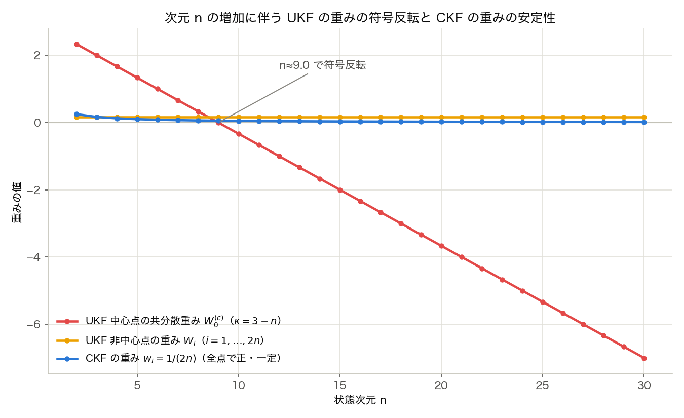
The red line (UKF’s central-point covariance weight) decreases monotonically with \(n\) , crosses zero at \(n=9\) , and then diverges in the negative direction. The orange line (UKF’s non-central weight, constant at \(1/6\) under this \(\kappa=3-n\) setting) and the blue line (CKF’s weight) both stay small and remain stably positive.
(2) Outright failure of sigma-point generation in high dimensions. Next, at state dimension \(n=20\) , we deliberately choose \(\kappa\) so that \(n+\kappa<0\) (setting \(\kappa=-(n+5)=-25\) ), giving \(n+\lambda=-5<0\) , and confirm that the matrix square root \(\sqrt{(n+\lambda)\mathbf P}\) required for UKF’s sigma-point generation no longer exists.
import numpy as np

np.random.seed(0)
n = 20
kappa = -(n + 5)
alpha, beta = 1.0, 2.0
lam = alpha**2 * (n + kappa) - n
print(f"n={n}, kappa={kappa}: n+kappa={n + kappa}, lambda={lam}, n+lambda={n + lam}")

# a random but positive-definite covariance matrix
A = np.random.randn(n, n) * 0.3
P = A @ A.T + np.eye(n) * 0.5
print("Is P positive definite:", np.all(np.linalg.eigvalsh(P) > 0))

# UKF: requires sqrt((n+lambda) P)
M_ukf = (n + lam) * P
eigs_ukf = np.linalg.eigvalsh(M_ukf)
print(f"Eigenvalue range of (n+lambda)P: [{eigs_ukf.min():.3f}, {eigs_ukf.max():.3f}]")
try:
    np.linalg.cholesky(M_ukf)
    print("UKF: Cholesky decomposition succeeded")
except np.linalg.LinAlgError as e:
    print(f"UKF: Cholesky decomposition FAILED -> {e}")

# CKF: sqrt(n P) always exists as long as P is positive definite
M_ckf = n * P
eigs_ckf = np.linalg.eigvalsh(M_ckf)
print(f"Eigenvalue range of nP: [{eigs_ckf.min():.3f}, {eigs_ckf.max():.3f}]")
L_ckf = np.linalg.cholesky(M_ckf)
print(f"CKF: Cholesky decomposition succeeded, shape={L_ckf.shape}")
Output:
n=20, kappa=-25: n+kappa=-5, lambda=-25.0, n+lambda=-5.0
Is P positive definite: True
Eigenvalue range of (n+lambda)P: [-35.120, -2.597]
UKF: Cholesky decomposition FAILED -> Matrix is not positive definite
Eigenvalue range of nP: [10.387, 140.480]
CKF: Cholesky decomposition succeeded, shape=(20, 20)
Even though \(\mathbf P\)
itself is positive definite, \((n+\lambda)\mathbf P\)
has all-negative eigenvalues because the scale factor \(n+\lambda=-5\)
is negative, so numpy.linalg.cholesky raises LinAlgError: Matrix is not positive definite, and UKF’s sigma-point generation fails outright. CKF’s cubature-point generation, by contrast, is a Cholesky decomposition of \(n\mathbf P\)
(\(n=20>0\)
), whose eigenvalues are guaranteed positive as long as \(\mathbf P\)
is positive definite, so it succeeds without issue even in 20 dimensions. This is a direct consequence of CKF having no tunable scaling parameter at all.
Related Articles
- Kalman Filter: Theory and Python Implementation - The linear Kalman filter that forms the foundation of CKF.
- Extended Kalman Filter (EKF): Theory and Python Implementation - Jacobian-based linearization approach for nonlinear systems.
- Unscented Kalman Filter (UKF): Nonlinear State Estimation Theory and Python Implementation - A sigma-point method in the same family as CKF.
- Particle Filter Python Implementation: Comparing Resampling Methods - Monte Carlo-based filtering for non-Gaussian distributions.
- Kalman Smoother (RTS Smoother): Theory and Python Implementation - Smoothing filter results using observations from all time steps.
- Kalman Smoother Comparison - Cross-method comparison of Kalman smoothing approaches that build on sigma-point filters such as the CKF.
References
- Arasaratnam, I., & Haykin, S. (2009). “Cubature Kalman Filters.” IEEE Transactions on Automatic Control, 54(6), 1254-1269.
- Jia, B., Xin, M., & Cheng, Y. (2013). “High-degree cubature Kalman filter.” Automatica, 49(2), 510-518.
- Katayama, T. (2011). “Basics of Nonlinear Kalman Filters.” Journal of SICE, 50(9), 638-643.