What is MPPI?
In the article on Cross-Entropy Method (CEM) , we introduced a method for iteratively optimizing the parameters of a sampling distribution in importance sampling.
Model Predictive Path Integral (MPPI) is a sampling-based model predictive control (MPC) algorithm grounded in stochastic optimal control theory. Although CEM and MPPI appear to take different approaches, they can be understood through a unified mathematical framework based on importance sampling and variational inference.
- CEM: “Hard” selection of elite samples (top \(P\) %)
- MPPI: “Soft” exponential weighting based on cost
Reference: Williams, G., et al. (2017). “Information Theoretic MPC for Model-Based Reinforcement Learning.” ICRA 2017.
Problem Setup
Consider a discrete-time stochastic dynamical system:
\[ \mathbf{x}_{t+1} = F(\mathbf{x}_t, \mathbf{u}_t) + \boldsymbol{\epsilon}_t, \quad \boldsymbol{\epsilon}_t \sim \mathcal{N}(\mathbf{0}, \boldsymbol{\Sigma}) \tag{1} \]where \(\mathbf{x}_t\) is the state, \(\mathbf{u}_t\) is the control input, and \(\boldsymbol{\epsilon}_t\) is the system noise.
The cost function for a control sequence \(\mathbf{U} = (\mathbf{u}_0, \mathbf{u}_1, \ldots, \mathbf{u}_{T-1})\) is defined as:
\[ J(\mathbf{U}) = \phi(\mathbf{x}_T) + \sum_{t=0}^{T-1} q(\mathbf{x}_t, \mathbf{u}_t) \tag{2} \]where \(\phi\) is the terminal cost and \(q\) is the stage cost.
Derivation of MPPI
Why does the optimal control distribution take the special exponential form \(\exp(-J/\lambda)\) ? Rather than accepting this as given, we derive it from first principles of stochastic optimal control.
Background: Linearizing the HJB Equation (Kappen’s Theory)
MPPI’s name — “Path Integral” — comes from Kappen’s (2005) theory of linearly solvable stochastic control. Consider a continuous-time, control-affine stochastic differential equation
\[ d\mathbf{x} = \mathbf{f}(\mathbf{x})\,dt + \mathbf{G}(\mathbf{x})\bigl(\mathbf{u}\,dt + d\boldsymbol{\omega}\bigr), \qquad d\boldsymbol{\omega} \sim \mathcal{N}(\mathbf{0}, \boldsymbol{\Sigma}\,dt) \] \[ \tag{P1} \]and a cost functional that is the sum of a terminal cost and a stage cost consisting of a state cost \(q(\mathbf{x})\) and a quadratic control cost \(\frac12 \mathbf{u}^T R \mathbf{u}\) :
\[ C(\mathbf{x}, t, \mathbf{u}(\cdot)) = \mathbb{E}\left[\phi(\mathbf{x}_T) + \int_t^T \left(q(\mathbf{x}_s) + \frac12 \mathbf{u}_s^T R \mathbf{u}_s\right) ds\right] \] \[ \tag{P2} \]The value function \(V(\mathbf{x}, t) = \min_{\mathbf{u}(\cdot)} C(\mathbf{x}, t, \mathbf{u}(\cdot))\) satisfies the Hamilton-Jacobi-Bellman (HJB) equation, which follows from Itô’s formula:
\[ -\partial_t V = \min_{\mathbf{u}} \left[ q(\mathbf{x}) + \frac12 \mathbf{u}^T R \mathbf{u} + (\nabla V)^T(\mathbf{f} + \mathbf{G}\mathbf{u}) + \frac12 \mathrm{tr}\bigl(\mathbf{G}\boldsymbol{\Sigma}\mathbf{G}^T \nabla^2 V\bigr)\right] \] \[ \tag{P3} \]The right-hand side is a convex quadratic in \(\mathbf{u}\) , so we can minimize analytically by setting the derivative to zero:
\[ \mathbf{u}^* = -R^{-1}\mathbf{G}^T \nabla V \tag{P4} \]Substituting back into (P3):
\[ -\partial_t V = q(\mathbf{x}) + (\nabla V)^T \mathbf{f} - \frac12 (\nabla V)^T \mathbf{G} R^{-1} \mathbf{G}^T \nabla V + \frac12 \mathrm{tr}\bigl(\mathbf{G}\boldsymbol{\Sigma}\mathbf{G}^T \nabla^2 V\bigr) \] \[ \tag{P5} \]This PDE contains a quadratic term in \(\nabla V\) and is therefore nonlinear — this is exactly why general stochastic optimal control problems cannot be solved analytically.
Kappen’s key move is to assume a specific relationship between the noise covariance and the control cost weighting (“the amount of noise the system is subject to must be proportional to how cheap control is”):
\[ \mathbf{G}\boldsymbol{\Sigma}\mathbf{G}^T = \lambda\, \mathbf{G} R^{-1} \mathbf{G}^T \tag{P6} \]Under this assumption, define the desirability function:
\[ \psi(\mathbf{x}, t) = \exp\left(-\frac{V(\mathbf{x}, t)}{\lambda}\right) \tag{P7} \]Since \(V = -\lambda \log \psi\) , the chain rule gives
\[ \begin{aligned} \partial_t V &= -\lambda\,\frac{\partial_t \psi}{\psi}, \qquad \nabla V = -\lambda\,\frac{\nabla \psi}{\psi}, \\ \nabla^2 V &= -\lambda\,\frac{\nabla^2 \psi}{\psi} + \lambda\,\frac{\nabla\psi (\nabla\psi)^T}{\psi^2} \end{aligned} \] \[ \tag{P8} \]Substituting these into (P5), the terms proportional to \(\nabla\psi(\nabla\psi)^T/\psi^2\) appear in two places — the expansion of \((\nabla V)^T\mathbf{G}R^{-1}\mathbf{G}^T\nabla V\) and the expansion of \(\mathrm{tr}(\mathbf{G}\boldsymbol{\Sigma}\mathbf{G}^T\nabla^2 V)\) — and their combined coefficient is exactly \(\mathbf{G}\boldsymbol{\Sigma}\mathbf{G}^T - \lambda\mathbf{G}R^{-1}\mathbf{G}^T\) . By assumption (P6), this is identically zero. In other words, the nonlinear term does not merely cancel between two pieces — Kappen’s assumption makes its coefficient vanish outright. What remains simplifies to:
\[ \partial_t \psi = -\mathbf{f}^T \nabla \psi - \frac12 \mathrm{tr}\bigl(\mathbf{G}\boldsymbol{\Sigma}\mathbf{G}^T \nabla^2 \psi\bigr) + \frac{q(\mathbf{x})}{\lambda}\psi \] \[ \tag{P9} \]With the boundary condition \(\psi(\mathbf{x}, T) = \exp(-\phi(\mathbf{x})/\lambda)\) , equation (P9) is linear in \(\psi\) . The nonlinear HJB equation (P5) has been transformed into a linear second-order PDE via the exponential transform (P7) together with the noise-cost matching condition (P6). This is why the result is called “linearly solvable stochastic control.”
The first two terms on the right-hand side of (P9) are exactly the generator \(\mathcal{L}\psi = \mathbf{f}^T\nabla\psi + \frac12\mathrm{tr}(\mathbf{G}\boldsymbol{\Sigma}\mathbf{G}^T\nabla^2\psi)\) of the uncontrolled (“passive”, \(\mathbf{u}=\mathbf{0}\) ) diffusion \(d\mathbf{x}=\mathbf{f}\,dt+\mathbf{G}\,d\boldsymbol{\omega}\) . So (P9) has the standard form \(\partial_t\psi + \mathcal{L}\psi - \frac{q(\mathbf{x})}{\lambda}\psi = 0\) , and by the Feynman-Kac theorem it can be represented as an expectation over paths of the passive diffusion:
\[ \psi(\mathbf{x}, t) = \mathbb{E}_{\text{passive}}\left[\left.\exp\left(-\frac1\lambda \int_t^T q(\mathbf{x}_s)\,ds - \frac1\lambda \phi(\mathbf{x}_T)\right) \right| \mathbf{x}_t = \mathbf{x}\right] \] \[ \tag{P10} \]This expectation is an integral over an infinite ensemble of random paths — a “path integral” — which is the origin of the name Path Integral Control. The optimal control law can be read off directly from the gradient of \(\psi\) :
\[ \mathbf{u}^*(\mathbf{x}, t) = -R^{-1}\mathbf{G}^T \nabla V = \lambda R^{-1}\mathbf{G}^T \nabla \log \psi(\mathbf{x}, t) \tag{P11} \]Connection to MPPI: MPPI is a Monte Carlo approximation of the expectation in (P10), replacing the analytic solution of the PDE with sampling. Drawing \(N\) rollouts from the passive dynamics (i.e. trajectories driven only by noise), evaluating the accumulated cost \(J(\mathbf{V}^{(i)})\) along each, and computing \(\frac1N\sum_i \exp(-J^{(i)}/\lambda)\) is nothing but an empirical estimate of \(\psi\) in (P10). The weighted-average update rule derived in the next section is exactly the procedure for recovering the optimal control (P11) from this estimate of \(\psi\) . In other words, the discrete-time, finite-horizon MPPI algorithm can be understood as a receding-horizon numerical recipe for solving Kappen’s continuous-time theory.
Optimal Control Distribution
In the stochastic optimal control framework, we treat the control sequence as a random variable and define the optimal control distribution as:
\[ p^*(\mathbf{V}) \propto \exp\left(-\frac{1}{\lambda} J(\mathbf{V})\right) \cdot p(\mathbf{V}) \tag{3} \]where \(\mathbf{V}\) is the noisy control sequence, \(\lambda > 0\) is the temperature parameter, and \(p(\mathbf{V})\) is the prior distribution (current sampling distribution). In the notation of the previous section, \(J(\mathbf{V})/\lambda\) corresponds — under the discrete-time approximation — to the continuous-time quantity \(-\log\psi\) ; equation (3) is precisely a reweighting of paths by the desirability function \(\psi\) .
The role of temperature \(\lambda\) :
- \(\lambda \to 0\) : Selects only the minimum-cost control sequence (hard selection)
- \(\lambda \to \infty\) : Weights all control sequences equally
Derivation via Variational Inference: Moment Projection (M-projection)
We cannot sample directly from \(p^*(\mathbf{V})\) in (3) — if we could, the optimal control problem would already be solved. Instead, we replace this with an approximation problem: find, within the same Gaussian family \(q(\mathbf{V}; \mathbf{U}) = \mathcal{N}(\mathbf{U}, \boldsymbol{\Sigma})\) as the current sampling policy, the distribution closest to \(p^*\) . Using KL divergence as the notion of “closeness,” we solve the following moment projection (M-projection):
\[ \hat{\mathbf{U}} = \operatorname*{arg\,min}_{\mathbf{U}}\ D_{\mathrm{KL}}\bigl(p^*(\mathbf{V}) \,\|\, q(\mathbf{V}; \mathbf{U})\bigr) \tag{3a} \](Note the direction is opposite to the mode-seeking I-projection, which minimizes \(D_{\mathrm{KL}}(q \| p^*)\) . I-projection generally has no closed form, whereas M-projection has a closed-form moment-matching solution for exponential-family distributions.)
Expanding with \(\boldsymbol{\Sigma}\) fixed and minimizing only over \(\mathbf{U}\) :
\[ D_{\mathrm{KL}}(p^* \| q) = -H[p^*] + \frac12\, \mathbb{E}_{p^*}\!\left[(\mathbf{V}-\mathbf{U})^T \boldsymbol{\Sigma}^{-1} (\mathbf{V}-\mathbf{U})\right] + \text{const.} \]Setting the gradient with respect to \(\mathbf{U}\) to zero gives \(\boldsymbol{\Sigma}^{-1}\mathbb{E}_{p^*}[\mathbf{V}-\mathbf{U}] = \mathbf{0}\) , i.e.
\[ \hat{\mathbf{U}} = \mathbb{E}_{p^*}[\mathbf{V}] \tag{3b} \]so moment matching is rigorously shown to be the optimal solution (an instance of the general exponential-family fact that KL projection onto a Gaussian always reduces to matching the first moment). Substituting \(p^*(\mathbf{V}) \propto \exp(-J(\mathbf{V})/\lambda)p(\mathbf{V})\) from (3):
\[ \hat{\mathbf{U}} = \frac{\displaystyle\int \mathbf{V}\exp\!\left(-\frac{J(\mathbf{V})}{\lambda}\right)p(\mathbf{V})\,d\mathbf{V}}{\displaystyle\int \exp\!\left(-\frac{J(\mathbf{V})}{\lambda}\right)p(\mathbf{V})\,d\mathbf{V}} \tag{3c} \]This integral cannot be evaluated in closed form, since \(J\) is a nonlinear functional of the dynamics rollout, but it is exactly an expectation under \(p(\mathbf{V})\) (the current sampling policy). Drawing \(N\) samples \(\mathbf{V}^{(i)} \sim p(\mathbf{V})\) and estimating this expectation by self-normalized importance sampling:
\[ \hat{\mathbf{U}} \approx \sum_{i=1}^N w^{(i)} \mathbf{V}^{(i)}, \qquad w^{(i)} = \frac{\exp(-J(\mathbf{V}^{(i)})/\lambda)}{\sum_{j=1}^N \exp(-J(\mathbf{V}^{(j)})/\lambda)} \tag{3d} \]This is exactly equations (4) and (5) below. In other words, MPPI’s weighted-average update rule is rigorously derivable as “a Monte Carlo estimate, via self-normalized importance sampling, of the moment projection of the optimal path distribution \(p^*\) onto the Gaussian family.” The label “variational inference as MPC” only makes precise sense once this specific projection direction (M-projection) and the Gaussian-family restriction are pinned down.
Weighted Control Update
We draw \(N\) samples \(\mathbf{V}^{(1)}, \ldots, \mathbf{V}^{(N)}\) from the prior \(p(\mathbf{V})\) and compute the cost \(J(\mathbf{V}^{(i)})\) for each.
The importance sampling weights are computed as (identical to (3d)):
\[ w^{(i)} = \frac{\exp\left(-\frac{1}{\lambda} J(\mathbf{V}^{(i)})\right)}{\sum_{j=1}^N \exp\left(-\frac{1}{\lambda} J(\mathbf{V}^{(j)})\right)} \tag{4} \]The optimal control input is obtained as a weighted average:
\[ \mathbf{u}_t^* = \sum_{i=1}^N w^{(i)} \mathbf{v}_t^{(i)} \tag{5} \]The Role of the Temperature Parameter \(\lambda\) : A Numerical Experiment
Theoretically, the weights \(w^{(i)}\) in (4) behave as follows:
- \(\lambda \to 0\) : Even a small cost difference \(J(\mathbf{V}^{(i)}) - J_{\min}\) is exponentially amplified, and the weight collapses onto the single lowest-cost sample (approaching hard selection).
- \(\lambda \to \infty\) : All samples receive nearly equal weight, and the update approaches a random average over the prior (broad exploration but no exploitation of information).
To quantify this concentration, we use the effective sample size (ESS) from importance sampling:
\[ \mathrm{ESS} = \frac{1}{\sum_{i=1}^N (w^{(i)})^2} \tag{6} \]ESS approaches \(N\) when weights are uniform, and approaches \(1\) when weight collapses onto a single sample. Below, we vectorize the rollout computation of this article’s Python implementation (see later) over samples using NumPy, fix \(N=500\) and random seed 42, and compare \(\lambda \in \{0.05, 0.2, 1.0, 5.0, 20.0\}\) , measuring the ESS at each step and the closed-loop cumulative cost.
import numpy as np

def dynamics_batch(x, u, dt=0.1):
    """Batched dynamics model. x: (N, 4), u: (N, 2) -> (N, 4)"""
    x_next = np.empty_like(x)
    x_next[:, 0] = x[:, 0] + x[:, 2] * dt
    x_next[:, 1] = x[:, 1] + x[:, 3] * dt
    x_next[:, 2] = x[:, 2] + u[:, 0] * dt
    x_next[:, 3] = x[:, 3] + u[:, 1] * dt
    return x_next

def stage_cost_batch(x, u, goal):
    dist = np.sum((x[:, :2] - goal) ** 2, axis=1)
    ctrl = 0.01 * np.sum(u**2, axis=1)
    return dist + ctrl

def terminal_cost_batch(x, goal):
    return 10.0 * np.sum((x[:, :2] - goal) ** 2, axis=1)

class MPPIControllerVec:
    """MPPI controller with vectorized rollouts for the experiments below.
    Mathematically identical to the original MPPIController; the only
    difference is evaluating the N samples as NumPy array operations
    instead of a Python for-loop (production MPPI implementations
    parallelize in exactly this way, typically on a GPU)."""
    def __init__(self, N, lam, T=20, n_ctrl=2, sigma=0.5, goal=np.array([5.0, 5.0])):
        self.N, self.lam, self.T, self.sigma, self.goal = N, lam, T, sigma, goal
        self.mu = np.zeros((T, n_ctrl))

    def compute_control(self, x0, rng):
        N, T = self.N, self.T
        noise = rng.standard_normal((N, T, self.mu.shape[1])) * self.sigma
        V = self.mu[np.newaxis, :, :] + noise

        x = np.tile(x0, (N, 1))
        costs = np.zeros(N)
        for t in range(T):
            costs += stage_cost_batch(x, V[:, t, :], self.goal)
            x = dynamics_batch(x, V[:, t, :])
        costs += terminal_cost_batch(x, self.goal)

        costs_shifted = costs - np.min(costs)
        weights = np.exp(-costs_shifted / self.lam)
        weights /= np.sum(weights)
        ess = 1.0 / np.sum(weights**2)  # Eq. (6)

        self.mu += np.sum(weights[:, np.newaxis, np.newaxis] * noise, axis=0)
        u_opt = self.mu[0].copy()
        self.mu = np.roll(self.mu, -1, axis=0)
        self.mu[-1] = 0.0
        return u_opt, ess


def run_episode(N, lam, n_steps=150, seed=42, goal=np.array([5.0, 5.0])):
    rng = np.random.default_rng(seed)
    x = np.array([0.0, 0.0, 0.0, 0.0])
    controller = MPPIControllerVec(N=N, lam=lam, goal=goal)
    ess_hist, total_cost = [], 0.0
    for _ in range(n_steps):
        u, ess = controller.compute_control(x, rng)
        ess_hist.append(ess)
        total_cost += stage_cost_batch(x[np.newaxis, :], u[np.newaxis, :], goal)[0]
        x = dynamics_batch(x[np.newaxis, :], u[np.newaxis, :])[0]
    return np.mean(ess_hist), total_cost


for lam in [0.05, 0.2, 1.0, 5.0, 20.0]:
    mean_ess, total_cost = run_episode(N=500, lam=lam, seed=42)
    print(f"lambda={lam:>6}: mean_ESS={mean_ess:6.1f} ({mean_ess/500*100:5.1f}% of N), "
          f"total_cost={total_cost:.2f}")
Results (random seed 42, \(N=500\) , 150 steps):
| \(\lambda\) | Mean ESS (% of N) | Cumulative cost | Step of first arrival |
|---|---|---|---|
| 0.05 | 3.5% | 709.41 | 28 |
| 0.2 | 16.3% | 709.94 | 30 |
| 1.0 | 52.1% | 723.20 | 41 |
| 5.0 | 81.7% | 748.72 | 40 |
| 20.0 | 86.8% | 878.48 | 35 |
As predicted by theory, ESS increases monotonically with \(\lambda\) (from 3.5% to 86.8% of \(N\) ), confirming that the weight mass spreads over more samples. On the other hand, cumulative cost is best when \(\lambda\) is small (709.41 at \(\lambda=0.05\) , the minimum, versus 878.48 at \(\lambda=20\) , the worst). For a smooth, unimodal quadratic cost like this one, aggressively trusting low-cost samples (small \(\lambda\) ) is advantageous. Conversely, when \(\lambda\) is too large, the informative signal from low-cost samples gets diluted by an update that is close to a uniform average over the prior, and performance degrades.
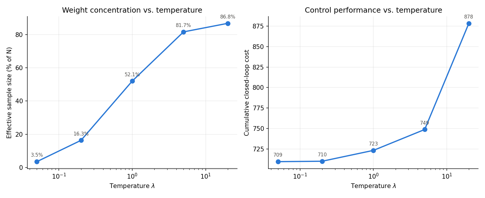
This is a trade-off between “breadth of exploration” and “precision of exploitation,” but note that the optimal point depends on the smoothness of the cost function. In the “Pitfalls of Cost Function Design” section below, we show that a property of the cost function itself (a lack of gradient information) can trigger the same mathematical mechanism (uniformization of weights), a failure mode that lowering \(\lambda\) alone cannot fix.
Comparison with CEM
Both CEM and MPPI share the structure of sampling control sequences from a current distribution and updating the distribution based on cost information.
CEM (Hard Selection)
CEM selects the top \(P\) % elite samples and updates the distribution parameters:
\[ \boldsymbol{\mu}_{\text{new}} = \frac{1}{|\mathcal{E}|} \sum_{i \in \mathcal{E}} \mathbf{V}^{(i)} \tag{7} \] \[ \boldsymbol{\Sigma}_{\text{new}} = \frac{1}{|\mathcal{E}|} \sum_{i \in \mathcal{E}} (\mathbf{V}^{(i)} - \boldsymbol{\mu}_{\text{new}})(\mathbf{V}^{(i)} - \boldsymbol{\mu}_{\text{new}})^T \tag{8} \]where \(\mathcal{E}\) is the set of elite samples.
MPPI (Soft Weighting)
MPPI uses all samples with exponential weights:
\[ \boldsymbol{\mu}_{\text{new}} = \sum_{i=1}^N w^{(i)} \mathbf{V}^{(i)} \tag{9} \]Unified Understanding: Both Are Moment Projections
As derived in (3a)-(3d), MPPI’s update rule (9) is “a moment projection onto the distribution reweighted by the weight function \(w(\mathbf{V}) \propto \exp(-J(\mathbf{V})/\lambda)\) .” CEM’s update rule (7)-(8) fits into exactly the same framework: replacing the weight function with a hard 0/1 indicator
\[ w_{\text{CEM}}(\mathbf{V}) \propto \mathbb{1}\bigl[J(\mathbf{V}) \le J_{(P)}\bigr] \](where \(J_{(P)}\) is the lower \(P\) -th percentile and \(\mathbb{1}[\cdot]\) is the indicator function) reproduces CEM’s update rule via exactly the same moment-projection argument as (3a)-(3d). The difference between CEM and MPPI thus reduces to a single choice: which weight function \(w(\mathbf{V})\) is used to approximate the same moment-projection problem onto \(p^*\) :
\[ \min_{\mathbf{U}}\ D_{\mathrm{KL}}\bigl(p_w(\mathbf{V}) \,\|\, \mathcal{N}(\mathbf{V}; \mathbf{U}, \boldsymbol{\Sigma})\bigr), \qquad p_w(\mathbf{V}) \propto w(\mathbf{V})\,p(\mathbf{V}) \tag{10} \]CEM takes \(w\) to be an indicator function (hard threshold); MPPI takes \(w\) to be an exponential (soft weighting). This unified view lets us state the relationship between the two more precisely. In the limit \(\lambda \to 0\) , the weights in (4) degenerate onto the single minimum-cost sample (weight 1 on the best of the \(N\) samples, 0 on the rest). This corresponds to the degenerate case of CEM with the elite count reduced to \(|\mathcal{E}|=1\) (a point estimate, with no variance update). For a general \(0 < P < 1\) , CEM’s top-\(P\) % selection uses a different weight function (indicator vs. exponential) than MPPI’s \(\lambda \to 0\) limit, so the two methods are best understood as “two distinct instances of the same framework” rather than one being an exact limit of the other.
| CEM | MPPI | |
|---|---|---|
| Weight function \(w(\mathbf{V})\) | Indicator \(\mathbb{1}[J \le J_{(P)}]\) | Exponential \(\exp(-J/\lambda)\) |
| Sample usage | Top \(P\) % only | All samples |
| Weighting | Uniform (0 or 1) | Exponential (continuous) |
| Parameters | Elite ratio \(P\) | Temperature \(\lambda\) |
| Variance update | Yes | No (typically) |
| Mathematical interpretation | Moment projection under a hard threshold | Moment projection under a Boltzmann weight |
MPPI Algorithm
Input: Initial control sequence μ = (μ_0, ..., μ_{T-1}), num samples N, temperature λ, noise variance Σ
Repeat:
  1. Sample N noisy control sequences:
     ε_t^(i) ~ N(0, Σ),  V^(i) = μ + ε^(i)
  2. Compute cost for each sample:
     J(V^(i)) = φ(x_T^(i)) + Σ_t q(x_t^(i), v_t^(i))
  3. Compute weights:
     w^(i) = exp(-J(V^(i))/λ) / Σ_j exp(-J(V^(j))/λ)
  4. Update control input:
     μ_t ← μ_t + Σ_i w^(i) ε_t^(i)
  5. Apply first control input μ_0 and shift the sequence
Python Implementation
We implement MPPI for a 2D goal-reaching problem.
Problem Definition
import numpy as np
import matplotlib.pyplot as plt

# ---- Problem setup ----
n_state = 4     # state dimension [x, y, vx, vy]
n_ctrl = 2      # control dimension [ax, ay]
dt = 0.1        # time step
T = 20          # prediction horizon
N = 500         # number of samples
lam = 1.0       # temperature parameter
sigma = 0.5     # control noise standard deviation
goal = np.array([5.0, 5.0])  # goal position

def dynamics(x, u):
    """Linear dynamics model (2D point mass)"""
    x_next = np.zeros(n_state)
    x_next[0] = x[0] + x[2] * dt  # px
    x_next[1] = x[1] + x[3] * dt  # py
    x_next[2] = x[2] + u[0] * dt  # vx
    x_next[3] = x[3] + u[1] * dt  # vy
    return x_next

def stage_cost(x, u):
    """Stage cost"""
    pos = x[:2]
    dist = np.sum((pos - goal)**2)
    ctrl = 0.01 * np.sum(u**2)
    return dist + ctrl

def terminal_cost(x):
    """Terminal cost"""
    pos = x[:2]
    return 10.0 * np.sum((pos - goal)**2)
MPPI Controller
class MPPIController:
    def __init__(self):
        # Initialize control sequence to zeros
        self.mu = np.zeros((T, n_ctrl))

    def compute_control(self, x0):
        """Compute optimal control input using MPPI"""
        # Step 1: Sample noisy control sequences
        noise = np.random.randn(N, T, n_ctrl) * sigma
        V = self.mu[np.newaxis, :, :] + noise  # (N, T, n_ctrl)

        # Step 2: Compute cost for each sample
        costs = np.zeros(N)
        for i in range(N):
            x = x0.copy()
            for t in range(T):
                costs[i] += stage_cost(x, V[i, t])
                x = dynamics(x, V[i, t])
            costs[i] += terminal_cost(x)

        # Step 3: Compute weights (Eq. 4)
        # Subtract minimum cost for numerical stability
        costs_shifted = costs - np.min(costs)
        weights = np.exp(-costs_shifted / lam)
        weights /= np.sum(weights)  # normalize

        # Step 4: Update control input (Eq. 5)
        weighted_noise = np.sum(
            weights[:, np.newaxis, np.newaxis] * noise, axis=0
        )
        self.mu += weighted_noise

        # Optimal control input (first time step)
        u_opt = self.mu[0].copy()

        # Shift control sequence for next time step
        self.mu = np.roll(self.mu, -1, axis=0)
        self.mu[-1] = 0.0  # set last element to zero

        return u_opt
Simulation
np.random.seed(42)

# Initial state
x = np.array([0.0, 0.0, 0.0, 0.0])
controller = MPPIController()

# Simulation
n_steps = 100
trajectory = [x.copy()]
controls = []

for step in range(n_steps):
    u = controller.compute_control(x)
    controls.append(u.copy())
    x = dynamics(x, u)
    trajectory.append(x.copy())

    # Check goal
    if np.linalg.norm(x[:2] - goal) < 0.1:
        print(f"Goal reached at step {step + 1}")
        break

trajectory = np.array(trajectory)
controls = np.array(controls)

# ---- Plot results ----
fig, axes = plt.subplots(1, 2, figsize=(14, 6))

# Trajectory
axes[0].plot(trajectory[:, 0], trajectory[:, 1], "b-o",
             markersize=3, label="MPPI trajectory")
axes[0].plot(*goal, "r*", markersize=15, label="Goal")
axes[0].plot(0, 0, "gs", markersize=10, label="Start")
axes[0].set_xlabel("x")
axes[0].set_ylabel("y")
axes[0].set_title("MPPI - Goal Reaching")
axes[0].legend()
axes[0].grid(True)
axes[0].set_aspect("equal")

# Control inputs
axes[1].plot(controls[:, 0], label="$a_x$")
axes[1].plot(controls[:, 1], label="$a_y$")
axes[1].set_xlabel("Step")
axes[1].set_ylabel("Control input")
axes[1].set_title("Control inputs over time")
axes[1].legend()
axes[1].grid(True)

plt.tight_layout()
plt.savefig("mppi_result.png", dpi=150)
plt.show()
Effect of Sample Count \(N\) (Numerical Experiment)
As the derivation in (3c)-(3d) shows, the weighted average is a Monte Carlo estimate of the integral \(\mathbb{E}_{p(\mathbf{V})}[\mathbf{V}\exp(-J(\mathbf{V})/\lambda)]\) . Monte Carlo estimation error generally decreases as \(O(1/\sqrt{N})\) , so we expect both the variance and (on average) the quality of control performance to improve as we increase \(N\) . To confirm this, we fix \(\lambda=1.0\) and run the closed-loop simulation across 10 random seeds for \(N \in \{20, 50, 100, 500, 2000\}\) .
import numpy as np

goal = np.array([5.0, 5.0])
dt, T, sigma = 0.1, 20, 0.5

def dynamics_batch(x, u):
    x_next = np.empty_like(x)
    x_next[:, 0] = x[:, 0] + x[:, 2] * dt
    x_next[:, 1] = x[:, 1] + x[:, 3] * dt
    x_next[:, 2] = x[:, 2] + u[:, 0] * dt
    x_next[:, 3] = x[:, 3] + u[:, 1] * dt
    return x_next

def stage_cost_batch(x, u):
    dist = np.sum((x[:, :2] - goal) ** 2, axis=1)
    ctrl = 0.01 * np.sum(u**2, axis=1)
    return dist + ctrl

def terminal_cost_batch(x):
    return 10.0 * np.sum((x[:, :2] - goal) ** 2, axis=1)

def run_episode(N, lam, seed, n_steps=150):
    rng = np.random.default_rng(seed)
    x = np.array([0.0, 0.0, 0.0, 0.0])
    mu = np.zeros((T, 2))
    total_cost = 0.0
    reached_step = None
    for step in range(n_steps):
        noise = rng.standard_normal((N, T, 2)) * sigma
        V = mu[np.newaxis, :, :] + noise
        xb = np.tile(x, (N, 1))
        costs = np.zeros(N)
        for t in range(T):
            costs += stage_cost_batch(xb, V[:, t, :])
            xb = dynamics_batch(xb, V[:, t, :])
        costs += terminal_cost_batch(xb)
        w = np.exp(-(costs - costs.min()) / lam)
        w /= w.sum()
        mu += np.sum(w[:, np.newaxis, np.newaxis] * noise, axis=0)
        u = mu[0].copy()
        total_cost += stage_cost_batch(x[np.newaxis, :], u[np.newaxis, :])[0]
        x = dynamics_batch(x[np.newaxis, :], u[np.newaxis, :])[0]
        mu = np.roll(mu, -1, axis=0)
        mu[-1] = 0.0
        if np.linalg.norm(x[:2] - goal) < 0.1 and reached_step is None:
            reached_step = step + 1
    final_dist = np.linalg.norm(x[:2] - goal)
    return final_dist, total_cost, (reached_step if reached_step is not None else n_steps)

for N in [20, 50, 100, 500, 2000]:
    dists, costs, reached = [], [], []
    for seed in range(10):
        d, c, r = run_episode(N=N, lam=1.0, seed=seed)
        dists.append(d)
        costs.append(c)
        reached.append(r)
    dists, costs, reached = np.array(dists), np.array(costs), np.array(reached)
    print(f"N={N:>5}: reached_step={reached.mean():.1f}+-{reached.std():.1f}, "
          f"final_dist={dists.mean():.4f}+-{dists.std():.4f}, "
          f"total_cost={costs.mean():.2f}+-{costs.std():.2f}")
Results (mean ± std over 10 seeds, 150 steps, \(\lambda=1.0\) ):
| \(N\) | Step of first arrival | Final distance error | Cumulative cost |
|---|---|---|---|
| 20 | 44.6 ± 2.8 | 0.0465 ± 0.0233 | 833.58 ± 24.91 |
| 50 | 45.0 ± 2.7 | 0.0334 ± 0.0103 | 789.53 ± 23.39 |
| 100 | 42.5 ± 1.7 | 0.0232 ± 0.0094 | 765.54 ± 15.97 |
| 500 | 40.5 ± 0.9 | 0.0154 ± 0.0091 | 723.27 ± 10.74 |
| 2000 | 39.3 ± 0.6 | 0.0073 ± 0.0032 | 697.11 ± 8.58 |
All conditions eventually reached the goal (distance below 0.1, 10/10), but increasing \(N\) from 20 to 2000 lowered the mean cumulative cost from 833.58 to 697.11 (about 16% better) while shrinking the standard deviation from 24.91 to 8.58 (roughly a factor of 3). This is consistent with the theoretical prediction that Monte Carlo estimation variance decreases with \(N\) . In practice, \(N\) should be chosen as a trade-off between compute budget (how many rollouts can be evaluated per control cycle) and the tolerance for variance in control performance.
Pitfalls of Cost Function Design: Divergence with Weak Gradient Information
MPPI’s weights (4) are determined by the relative cost difference \(J(\mathbf{V}^{(i)}) - J_{\min}\) . So if the cost function is nearly constant over some region (little or no gradient information, or locally flat), the cost differences between samples in that region are nearly zero, and the weights become nearly uniform. This is mathematically the exact same phenomenon (uniformization of weights) as the “\(\lambda\) too large” case from the previous section, except triggered by a property of the cost function rather than the temperature.
To confirm this, we compare the usual quadratic cost (stage_cost_batch) against a “plateau” cost that is constant (zero gradient) outside a radius of 1.0 from the goal, and quadratic only inside that radius:
import numpy as np

goal = np.array([5.0, 5.0])
dt, T, sigma, lam, N = 0.1, 20, 0.5, 1.0, 500

def dynamics_batch(x, u):
    x_next = np.empty_like(x)
    x_next[:, 0] = x[:, 0] + x[:, 2] * dt
    x_next[:, 1] = x[:, 1] + x[:, 3] * dt
    x_next[:, 2] = x[:, 2] + u[:, 0] * dt
    x_next[:, 3] = x[:, 3] + u[:, 1] * dt
    return x_next

def stage_cost_quadratic(x, u):
    return np.sum((x[:, :2] - goal) ** 2, axis=1) + 0.01 * np.sum(u**2, axis=1)

def terminal_cost_quadratic(x):
    return 10.0 * np.sum((x[:, :2] - goal) ** 2, axis=1)

def stage_cost_flat(x, u):
    """Constant value 50 (zero gradient) outside radius 1.0 of the goal,
    quadratic only inside."""
    dist = np.linalg.norm(x[:, :2] - goal, axis=1)
    ctrl = 0.01 * np.sum(u**2, axis=1)
    return np.where(dist <= 1.0, 50.0 * dist**2, 50.0) + ctrl

def terminal_cost_flat(x):
    dist = np.linalg.norm(x[:, :2] - goal, axis=1)
    return np.where(dist <= 1.0, 500.0 * dist**2, 500.0)

def run_episode(stage_cost, terminal_cost, seed, n_steps=150):
    rng = np.random.default_rng(seed)
    x = np.array([0.0, 0.0, 0.0, 0.0])
    mu = np.zeros((T, 2))
    ess_hist = []
    for _ in range(n_steps):
        noise = rng.standard_normal((N, T, 2)) * sigma
        V = mu[np.newaxis, :, :] + noise
        xb = np.tile(x, (N, 1))
        costs = np.zeros(N)
        for t in range(T):
            costs += stage_cost(xb, V[:, t, :])
            xb = dynamics_batch(xb, V[:, t, :])
        costs += terminal_cost(xb)
        w = np.exp(-(costs - costs.min()) / lam)
        w /= w.sum()
        ess_hist.append(1.0 / np.sum(w**2))
        mu += np.sum(w[:, np.newaxis, np.newaxis] * noise, axis=0)
        u = mu[0].copy()
        x = dynamics_batch(x[np.newaxis, :], u[np.newaxis, :])[0]
        mu = np.roll(mu, -1, axis=0)
        mu[-1] = 0.0
    final_dist = np.linalg.norm(x[:2] - goal)
    return final_dist, np.mean(ess_hist)

for label, sc, tc in [("quadratic (baseline)", stage_cost_quadratic, terminal_cost_quadratic),
                       ("flat/plateau (adversarial)", stage_cost_flat, terminal_cost_flat)]:
    dists, ess_fracs = [], []
    for seed in range(10):
        d, ess = run_episode(sc, tc, seed=seed)
        dists.append(d)
        ess_fracs.append(ess / N * 100)
    dists = np.array(dists)
    n_success = int(np.sum(dists < 0.1))
    print(f"{label:>28}: success={n_success}/10, final_dist={dists.mean():.4f}+-{dists.std():.4f}, "
          f"mean_ESS={np.mean(ess_fracs):.2f}% of N")
Results (10 seeds, \(N=500\) , \(\lambda=1.0\) , 150 steps):
| Cost function | Success rate | Final distance error | Mean ESS (% of N) |
|---|---|---|---|
| Quadratic (baseline) | 10/10 | 0.0154 ± 0.0091 | 51.9 ± 0.18% |
| Plateau (no gradient) | 0/10 | 6.9813 ± 0.6629 | 99.95 ± 0.0003% |
The result is dramatic. The quadratic cost reached the goal in all 10 seeds (final distance error 0.0154), while the plateau cost failed to reach the goal in all 10 seeds, stalling at an average distance of 6.98 from the goal after 150 steps. The mean ESS confirms the mechanism: 51.9% for the quadratic cost versus 99.95% for the plateau cost — weights are almost perfectly uniform, essentially equal to \(N\) . This is exactly the same mathematical consequence as the \(\lambda \to \infty\) limit from the previous section (ESS approaching \(N\) in Eq. (6)).
The mechanism is as follows: while the robot is outside the radius-1.0 region, every rollout incurs almost the same constant cost (around the plateau value of 50, differing only slightly through the control cost), so \(J(\mathbf{V}^{(i)}) - J_{\min}\) stays small relative to \(\lambda\) and the weights become nearly uniform. The weighted average in (3d) then collapses to nearly the prior mean (a simple average of zero-mean noise), and the control update degenerates into essentially a random walk. The robot receives no meaningful drive toward the goal and wanders indefinitely in the plateau region. Crucially, this failure cannot be fixed by lowering \(\lambda\) , since the problem is that the cost function itself carries no gradient information — not that the temperature is miscalibrated. The practical lesson is that cost function design is the single most important factor governing the performance of sampling-based optimizers like MPPI: dense (ideally smooth and monotonic) gradient information toward the goal must be built into the cost function itself.
Recent Research Trends (2023 and Beyond)
While MPPI originated in robotics, research on both its applications and extensions has remained active since 2023.
- Real-time whole-body control of legged robots: Alvarez-Padilla et al. (2024) report running MPPI directly on hardware in real time for the whole-body dynamics of legged robots, including contact models, without any offline training. Because MPPI requires no gradients and parallelizes easily, it remains stable even with non-smooth dynamics and cost functions involving contact.
- Integration with learned neural networks: In autonomous driving, Ryu et al. (2025) propose IANN-MPPI, which incorporates a neural-network-based prior and interaction-aware cost design that accounts for surrounding vehicles into the MPPI framework. As this article’s experiments show, the paucity of gradient information in a cost function can severely degrade MPPI’s performance, so the growing trend of learning the cost function or the sampling distribution itself from data is consistent with the edge-case results demonstrated here.
- Hybridization with CEM for improved sample efficiency: As our sample-count experiment showed, MPPI’s performance is sensitive to \(N\) . Recent work has explored hybrid methods that combine elite selection (as in CEM) with MPPI to improve effective sample efficiency, with reported applications to gait optimization for legged robots.
All of these lines of research build on the basic principles derived in this article — the weighted Monte Carlo approximation in (3d), the ESS-based measure of weight concentration in (6), and the central importance of gradient information in cost function design. In real systems with substantial uncertainty, practical implementation choices like these, not just the theoretical derivation, determine how well the method works in practice.
Related Articles
- Simulated Annealing: Theory and Python Implementation - A stochastic search-based optimization method similar to MPPI.
- Bayesian Optimization: Fundamentals and Python Implementation - Efficient surrogate model-based optimization.
- Genetic Algorithms: Fundamentals and Python Implementation - Evolutionary computation-based metaheuristics.
- PID Control in Python: Simulation and Tuning - Classical control method for comparison with MPPI.
- Cross-Entropy Method: A Practical Monte Carlo Optimization Technique - The CEM counterpart with hard elite selection; both methods share the same importance-sampling foundation.
- Particle Swarm Optimization (PSO): Theory and Python Implementation - Another population-based optimizer; contrast PSO’s velocity/position update with MPPI’s cost-weighted averaging.
- Particle Filter: Resampling Strategies in Python - Same importance-sampling framework as MPPI’s soft weighting, applied to state estimation rather than control.
- Gaussian Process Regression: Theory and Python Implementation - GP surrogate alternative when each rollout is expensive — contrasts with MPPI’s mass-sampling strategy.
- Extended Kalman Filter (EKF): Theory and Python Implementation - Representative state-estimation method used alongside MPPI; clarifies the state-estimation + sampling-control combination.
- Monte Carlo Optimization Methods Comparison (CEM/SA/GA/MPPI/PSO) - Hub article organizing five Monte Carlo optimizers including MPPI under a common sample/evaluate/update skeleton, showing how MPPI’s soft weighting connects to the other methods.
References
- Kappen, H. J. (2005). “Linear Theory for Control of Nonlinear Stochastic Systems.” Physical Review Letters, 95(20), 200201.
- Kappen, H. J. (2005). “Path Integrals and Symmetry Breaking for Optimal Control Theory.” Journal of Statistical Mechanics: Theory and Experiment, 2005(11), P11011.
- Theodorou, E., Buchli, J., & Schaal, S. (2010). “A Generalized Path Integral Control Approach to Reinforcement Learning.” Journal of Machine Learning Research, 11, 3137-3181.
- Williams, G., Aldrich, A., & Theodorou, E. A. (2017). “Model Predictive Path Integral Control: From Theory to Parallel Computation.” Journal of Guidance, Control, and Dynamics, 40(2), 344-357.
- Williams, G., et al. (2017). “Information Theoretic MPC for Model-Based Reinforcement Learning.” ICRA 2017.
- Alvarez-Padilla, J., Zhang, J. Z., Kwok, S., Dolan, J. M., & Manchester, Z. (2024). “Real-Time Whole-Body Control of Legged Robots with Model-Predictive Path Integral Control.” arXiv:2409.10469.
- Ryu, K., Sung, M., Gupta, P., D’sa, J., Tariq, F. M., Isele, D., & Bae, S. (2025). “IANN-MPPI: Interaction-Aware Neural Network-Enhanced Model Predictive Path Integral Approach for Autonomous Driving.” arXiv:2507.11940.
- Rubinstein, R. Y., & Kroese, D. P. (2013). The Cross-Entropy Method. Springer.