What is Bayesian Optimization?
Bayesian optimization is a method for global optimization of expensive-to-evaluate black-box functions. It targets problems of the form:
\[ \mathbf{x}^* = \arg\min_{\mathbf{x} \in \mathcal{X}} f(\mathbf{x}) \tag{1} \]where \(f\) has no analytical gradient and each evaluation incurs a significant cost in time or resources. Common applications include hyperparameter tuning for machine learning models, experimental design, and materials discovery.
Bayesian optimization consists of two components:
- Surrogate model: A probabilistic model that approximates the objective function (typically a Gaussian process)
- Acquisition function: A criterion that determines which point to evaluate next
By building a surrogate from a small set of observations and sequentially selecting points that maximize the acquisition function, Bayesian optimization explores the search space efficiently.
Gaussian Process Regression
Kernel Functions
A Gaussian process (GP) defines a prior distribution over functions. A GP is fully specified by a mean function \(m(\mathbf{x})\) and a kernel function \(k(\mathbf{x}, \mathbf{x}')\) :
\[ f(\mathbf{x}) \sim \mathcal{GP}(m(\mathbf{x}), k(\mathbf{x}, \mathbf{x}')) \tag{2} \]The most widely used kernel is the RBF (Radial Basis Function) kernel, also known as the squared exponential kernel:
\[ k(\mathbf{x}, \mathbf{x}') = \sigma_f^2 \exp\left(-\frac{\|\mathbf{x} - \mathbf{x}'\|^2}{2l^2}\right) \tag{3} \]where \(\sigma_f^2\) is the output variance and \(l\) is the length-scale parameter. Larger values of \(l\) produce smoother functions.
Posterior Distribution
Given \(n\) observations \(\mathcal{D} = \{(\mathbf{x}_i, y_i)\}_{i=1}^n\) with observation noise \(\sigma_n^2\) , the predictive distribution at a new input \(\mathbf{x}_*\) is:
\[ \mu(\mathbf{x}_*) = \mathbf{k}_*^T (\mathbf{K} + \sigma_n^2 \mathbf{I})^{-1} \mathbf{y} \tag{4} \] \[ \sigma^2(\mathbf{x}_*) = k(\mathbf{x}_*, \mathbf{x}_*) - \mathbf{k}_*^T (\mathbf{K} + \sigma_n^2 \mathbf{I})^{-1} \mathbf{k}_* \tag{5} \]where:
- \(\mathbf{K}\) is the \(n \times n\) kernel matrix with \(K_{ij} = k(\mathbf{x}_i, \mathbf{x}_j)\)
- \(\mathbf{k}_* = [k(\mathbf{x}_1, \mathbf{x}_*), \ldots, k(\mathbf{x}_n, \mathbf{x}_*)]^T\)
- \(\mathbf{y} = [y_1, \ldots, y_n]^T\)
Equation (4) gives the predictive mean, and Equation (5) gives the predictive uncertainty. The variance \(\sigma^2\) shrinks in regions dense with data and grows in regions with sparse observations.
Acquisition Functions
Acquisition functions decide where to sample next. They balance exploitation (regions with low predicted mean) and exploration (regions with high uncertainty).
Expected Improvement (EI)
EI maximizes the expected improvement over the current best observed value \(f(\mathbf{x}^+)\) :
\[ \text{EI}(\mathbf{x}) = \mathbb{E}[\max(f(\mathbf{x}^+) - f(\mathbf{x}), 0)] \tag{6} \]Under the GP predictive distribution, EI admits a closed-form expression:
\[ \text{EI}(\mathbf{x}) = (\mu(\mathbf{x}^+) - \mu(\mathbf{x}) - \xi) \Phi(Z) + \sigma(\mathbf{x}) \phi(Z) \tag{7} \] \[ Z = \frac{\mu(\mathbf{x}^+) - \mu(\mathbf{x}) - \xi}{\sigma(\mathbf{x})} \tag{8} \]where \(\Phi\) and \(\phi\) are the CDF and PDF of the standard normal distribution, and \(\xi \geq 0\) is a parameter that encourages exploration. For minimization, \(f(\mathbf{x}^+)\) is the current minimum observation.
Deriving EI (proof of Eqs. 7-8)
Equation (6) cannot be evaluated directly as an expectation, so we turn it into a closed form using properties of the GP posterior. Define the improvement as
\[ I(\mathbf{x}) = \max(f(\mathbf{x}^+) - f(\mathbf{x}), 0) \tag{11} \]Since the GP posterior gives \(f(\mathbf{x}) \sim \mathcal{N}(\mu(\mathbf{x}), \sigma^2(\mathbf{x}))\) , writing \(u\) for a realization of \(f(\mathbf{x})\) , the expectation becomes the integral
\[ \text{EI}(\mathbf{x}) = \int_{-\infty}^{f(\mathbf{x}^+)} (f(\mathbf{x}^+) - u) \, \varphi(u) \, du \tag{12} \]where \(\varphi\) is the density of a normal distribution with mean \(\mu(\mathbf{x})\) and variance \(\sigma^2(\mathbf{x})\) . Substituting the standardized variable \(z = (u - \mu(\mathbf{x})) / \sigma(\mathbf{x})\) , the upper limit becomes \(Z = (f(\mathbf{x}^+) - \mu(\mathbf{x})) / \sigma(\mathbf{x})\) , giving
\[ \text{EI}(\mathbf{x}) = \int_{-\infty}^{Z} \big(f(\mathbf{x}^+) - \mu(\mathbf{x}) - \sigma(\mathbf{x}) z\big) \, \phi(z) \, dz \tag{13} \]where \(\phi\) is the standard normal density. Splitting the integral into two terms:
\[ \text{EI}(\mathbf{x}) = (f(\mathbf{x}^+) - \mu(\mathbf{x})) \int_{-\infty}^{Z} \phi(z) \, dz \; - \; \sigma(\mathbf{x}) \int_{-\infty}^{Z} z \, \phi(z) \, dz \tag{14} \]The first integral is, by definition, the standard normal CDF, so it equals \(\Phi(Z)\) . For the second, the derivative identity \(\frac{d}{dz}[-\phi(z)] = z \phi(z)\) shows that \(-\phi(z)\) is an antiderivative, so
\[ \int_{-\infty}^{Z} z \, \phi(z) \, dz = \big[-\phi(z)\big]_{-\infty}^{Z} = -\phi(Z) \tag{15} \](using \(\phi(z) \to 0\) as \(z \to -\infty\) ). Substituting back into Eq. (14):
\[ \text{EI}(\mathbf{x}) = (f(\mathbf{x}^+) - \mu(\mathbf{x})) \, \Phi(Z) + \sigma(\mathbf{x}) \, \phi(Z) \]which is exactly Eq. (7). Introducing the exploration term \(\xi \geq 0\) by replacing \(f(\mathbf{x}^+)\) with \(f(\mathbf{x}^+) - \xi\) yields the complete form in Eqs. (7)-(8). \(\xi\) raises the bar for what counts as an “improvement,” so larger \(\xi\) pushes EI toward more exploration.
Upper Confidence Bound (UCB)
For minimization, we use the Lower Confidence Bound variant:
\[ \text{UCB}(\mathbf{x}) = \mu(\mathbf{x}) - \kappa \sigma(\mathbf{x}) \tag{9} \]The parameter \(\kappa > 0\) controls the exploration–exploitation trade-off. Larger \(\kappa\) favors exploration.
Probability of Improvement (PI)
PI maximizes the probability of improving upon the current best value:
\[ \text{PI}(\mathbf{x}) = \Phi\left(\frac{\mu(\mathbf{x}^+) - \mu(\mathbf{x}) - \xi}{\sigma(\mathbf{x})}\right) \tag{10} \]PI is simple to compute but ignores the magnitude of improvement, which can lead to premature convergence to local optima.
Extension: Thompson Sampling as a Fourth Option
EI, UCB, and PI all plug the GP’s predictive mean and variance into an explicit formula to pick the next point. A different approach is Thompson Sampling, which instead draws one function from the posterior and directly picks that sample’s minimizer (or maximizer, for maximization problems) as the next evaluation point. We derive it from first principles in the multi-armed bandit setting and implement it combined with a Gaussian process as GP-TS, with a measured comparison against the EI acquisition function from this article, in https://yuhi-sa.github.io/en/posts/20260729_thompson_sampling/1/.
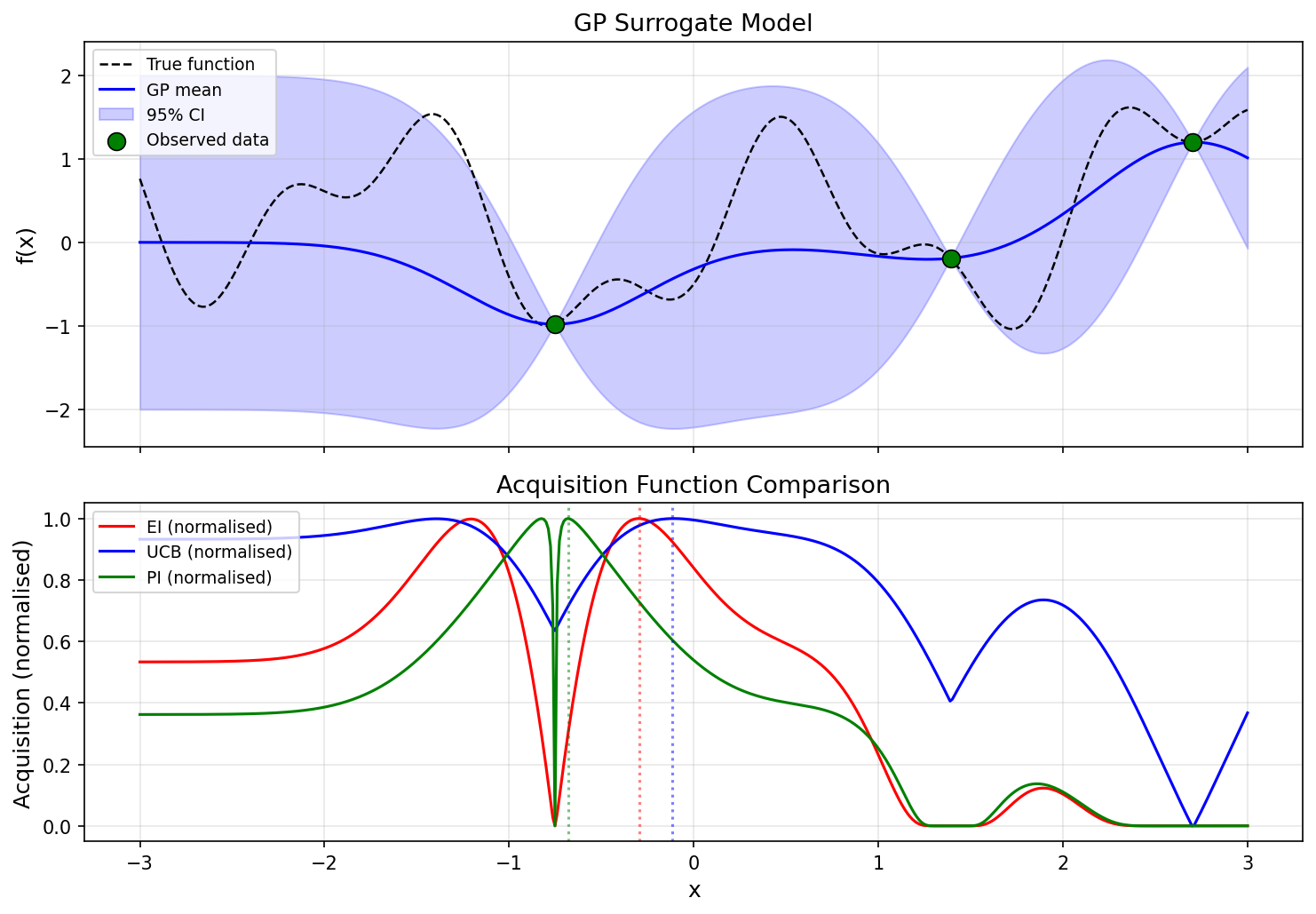
The figure below compares how the three acquisition functions suggest different exploration strategies for the same GP surrogate.
Python Implementation
Gaussian Process Class
We implement GP regression from scratch using NumPy and SciPy.
import numpy as np
from scipy.stats import norm

class GaussianProcess:
    def __init__(self, length_scale=1.0, signal_var=1.0, noise_var=1e-6):
        self.l = length_scale
        self.sf2 = signal_var
        self.sn2 = noise_var
        self.X_train = None
        self.y_train = None
        self.K_inv = None

    def kernel(self, X1, X2):
        """RBF kernel (Eq. 3)"""
        dist_sq = np.sum(X1**2, axis=1, keepdims=True) \
                  - 2.0 * X1 @ X2.T \
                  + np.sum(X2**2, axis=1)
        return self.sf2 * np.exp(-0.5 * dist_sq / self.l**2)

    def fit(self, X, y):
        """Fit the GP to observed data"""
        self.X_train = X.copy()
        self.y_train = y.copy()
        K = self.kernel(X, X) + self.sn2 * np.eye(len(X))
        self.K_inv = np.linalg.inv(K)

    def predict(self, X_new):
        """Predictive mean and variance at new points (Eqs. 4, 5)"""
        k_star = self.kernel(self.X_train, X_new)
        mu = k_star.T @ self.K_inv @ self.y_train
        var = self.sf2 - np.diag(k_star.T @ self.K_inv @ k_star)
        var = np.maximum(var, 1e-10)
        return mu, var
Acquisition Functions
def expected_improvement(mu, var, y_best, xi=0.01):
    """Expected Improvement (Eqs. 7, 8)"""
    sigma = np.sqrt(var)
    with np.errstate(divide="ignore", invalid="ignore"):
        Z = (y_best - mu - xi) / sigma
        ei = (y_best - mu - xi) * norm.cdf(Z) + sigma * norm.pdf(Z)
        ei[sigma < 1e-10] = 0.0
    return ei

def upper_confidence_bound(mu, var, kappa=2.0):
    """UCB for minimization (LCB) (Eq. 9)"""
    sigma = np.sqrt(var)
    return mu - kappa * sigma

def probability_of_improvement(mu, var, y_best, xi=0.01):
    """Probability of Improvement (Eq. 10)"""
    sigma = np.sqrt(var)
    with np.errstate(divide="ignore", invalid="ignore"):
        Z = (y_best - mu - xi) / sigma
        pi = norm.cdf(Z)
        pi[sigma < 1e-10] = 0.0
    return pi
Bayesian Optimization Loop
def bayesian_optimization(f, bounds, n_init=3, n_iter=15,
                          acq_func="ei"):
    """Main Bayesian optimization loop"""
    # Random initial samples
    X_init = np.random.uniform(bounds[0], bounds[1],
                               size=(n_init, 1))
    y_init = np.array([f(x) for x in X_init]).reshape(-1)

    gp = GaussianProcess(length_scale=0.5, signal_var=1.0,
                         noise_var=1e-6)
    X_sample = X_init.copy()
    y_sample = y_init.copy()

    # Optimization loop
    for i in range(n_iter):
        gp.fit(X_sample, y_sample)

        # Evaluate acquisition function over candidate points
        X_cand = np.linspace(bounds[0], bounds[1], 500).reshape(-1, 1)
        mu, var = gp.predict(X_cand)
        y_best = np.min(y_sample)

        if acq_func == "ei":
            acq = expected_improvement(mu, var, y_best)
            x_next = X_cand[np.argmax(acq)]
        elif acq_func == "ucb":
            acq = upper_confidence_bound(mu, var)
            x_next = X_cand[np.argmin(acq)]
        elif acq_func == "pi":
            acq = probability_of_improvement(mu, var, y_best)
            x_next = X_cand[np.argmax(acq)]

        # Evaluate and add the new point
        y_next = f(x_next.reshape(1, -1))
        X_sample = np.vstack([X_sample, x_next.reshape(1, -1)])
        y_sample = np.append(y_sample, y_next)

    return X_sample, y_sample, gp
1D Optimization Demo
We use a non-convex test function with multiple local minima to demonstrate Bayesian optimization.
import matplotlib.pyplot as plt

def test_function(x):
    """Test function with multiple local minima"""
    return np.sin(3 * x) + x**2 * 0.1 - 0.5 * np.cos(7 * x)

np.random.seed(42)
bounds = (-3.0, 3.0)
X_sample, y_sample, gp = bayesian_optimization(
    test_function, bounds, n_init=3, n_iter=12, acq_func="ei"
)

# Plot the results
X_plot = np.linspace(bounds[0], bounds[1], 300).reshape(-1, 1)
y_true = np.array([test_function(x) for x in X_plot])
mu, var = gp.predict(X_plot)
sigma = np.sqrt(var)

fig, axes = plt.subplots(2, 1, figsize=(10, 8))

# GP surrogate
axes[0].plot(X_plot, y_true, "k--", label="True function")
axes[0].plot(X_plot, mu, "b-", label="GP mean")
axes[0].fill_between(X_plot.ravel(), mu - 2*sigma, mu + 2*sigma,
                     alpha=0.2, color="blue", label="95% CI")
axes[0].scatter(X_sample[:3], y_sample[:3],
                c="green", s=80, zorder=5, label="Initial points")
axes[0].scatter(X_sample[3:], y_sample[3:],
                c="red", s=80, zorder=5, label="BO samples")
axes[0].set_xlabel("x")
axes[0].set_ylabel("f(x)")
axes[0].set_title("Bayesian Optimization with GP Surrogate")
axes[0].legend()
axes[0].grid(True)

# EI acquisition function
acq_ei = expected_improvement(mu, var, np.min(y_sample))
axes[1].plot(X_plot, acq_ei, "r-", label="EI")
axes[1].set_xlabel("x")
axes[1].set_ylabel("EI(x)")
axes[1].set_title("Expected Improvement")
axes[1].legend()
axes[1].grid(True)

plt.tight_layout()
plt.savefig("bayesian_optimization_result.png", dpi=150)
plt.show()

best_idx = np.argmin(y_sample)
print(f"Best x: {X_sample[best_idx].item():.4f}")
print(f"Best f(x): {y_sample[best_idx]:.4f}")
print(f"Total evaluations: {len(y_sample)}")
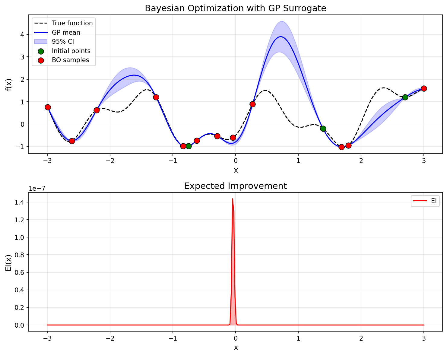
The GP predictive mean (blue line) converges toward the true function (dashed black line), while the confidence interval (blue band) narrows near observed data. The EI acquisition function takes large values in regions where uncertainty is high and improvement is expected, automatically balancing exploration and exploitation.
Actual Run Results
We executed the code above (verified with numpy 2.4.2, scipy 1.18.0, matplotlib 3.10.8). The optimization loop with the EI acquisition function printed:
Best x: 1.6894
Best f(x): -1.0210
Total evaluations: 15
The true global minimum of the test function, located by a dense grid search over 2,000,001 points, is \(\mathbf{x}^* = 1.723911\) , \(f(\mathbf{x}^*) = -1.038189\) (this exhaustive check is only possible because the test function is cheap to evaluate for verification purposes – it is not available for a real black-box objective). The regret of the EI solution after 15 evaluations (3 initial + 12 loop iterations) is therefore \(\lvert -1.0210 - (-1.038189) \rvert \approx 0.0172\) .
Re-running with the same seed and initial points but acq_func="ucb" and acq_func="pi" gives:
| Acquisition | Best x | Best f(x) | Regret (vs. true optimum) |
|---|---|---|---|
| EI | 1.6894 | -1.0210 | 0.0172 |
| UCB | 1.7014 | -1.0308 | 0.0074 |
| PI | 1.7134 | -1.0366 | 0.0016 |
The figure below shows the best-so-far value at each iteration for the three methods.
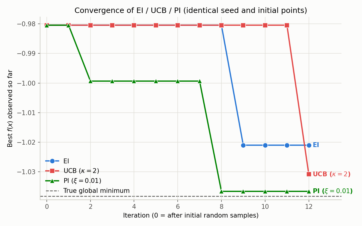
In this particular run, PI converges fastest and closest to the true optimum – but as discussed below, this is a single-seed result and does not generalize. PI maximizes only the probability of improvement, ignoring its magnitude, so once it locates a good local basin it tends to exploit it heavily; here that happened to pay off for this test function and seed. Averaged over many objectives and seeds, EI (which weighs the magnitude of improvement) and UCB (which carries a theoretical regret bound) are generally considered the more robust choices (Shahriari et al., 2016).
Practical Caveats and Edge Cases
The following pitfalls are easy to miss when translating the textbook formulas directly into code.
1. Numerical singularity as \(\sigma(\mathbf{x}) \to 0\)
At and near already-observed points, the predictive variance \(\sigma^2(\mathbf{x})\)
is nearly zero. The ratio \(Z\)
in Eq. (8) then divides by (near) zero, producing NaN/Inf if implemented naively. Our code suppresses the divide-by-zero warning with np.errstate and explicitly masks with ei[sigma < 1e-10] = 0.0. This matches the correct mathematical limit – \(\text{EI} \to 0\)
as \(\sigma \to 0^+\)
, since there is no room left for improvement where uncertainty vanishes. Skipping this mask can make the acquisition-function maximizer accidentally select a NaN.
2. Ill-conditioning of the kernel matrix
GaussianProcess.fit computes the inverse directly via np.linalg.inv(K). When observed points cluster closely, the condition number of \(\mathbf{K}\)
degrades sharply and the matrix inversion becomes numerically unstable (floating-point error can even make the predictive variance negative). Production libraries (e.g., scikit-learn’s GaussianProcessRegressor) use a Cholesky factorization (scipy.linalg.cho_factor / cho_solve) instead of forming the inverse explicitly, which is numerically far more stable. Our from-scratch implementation is simplified for pedagogical clarity (see
Gaussian Process Regression in Practice
for the Cholesky-based approach).
3. Scale-dependence of \(\xi\) (EI/PI) and \(\kappa\) (UCB)
\(\xi\) acts as an absolute offset on the scale of \(f(\mathbf{x})\) . As the objective’s range changes, the appropriate \(\xi\) changes too, so in practice it is safer to scale it by the observed standard deviation (e.g., \(\xi = 0.01 \times \text{std}(y)\) ). \(\kappa\) has a similar issue: the theoretical regret guarantee for GP-UCB requires scheduling \(\kappa\) with the iteration count \(t\) :
\[ \kappa_t = \sqrt{2 \log\left(\frac{t^{d/2+2} \pi^2}{3\delta}\right)} \tag{16} \](where \(d\) is the input dimension and \(\delta\) is the failure probability; Srinivas et al., 2010). Our demo used a fixed \(\kappa=2\) , a common practical simplification for short runs, but it does not retain the theoretical no-regret guarantee.
4. Don’t generalize from a single seed
As shown above, running EI, UCB, and PI with the same seed (seed=42) and the same initial points for 12 iterations, PI reached the best value. But concluding “PI is better” from a single run is unjustified. A statistically valid comparison requires averaging over many seeds and multiple test functions (varying multimodality and dimensionality).
5. The acquisition function’s own optimization is non-convex
Our implementation “optimizes” the acquisition function by evaluating it on a fixed 500-point grid via np.linspace and taking the argmax. This crude approach is tolerable only because the problem is one-dimensional – the number of grid points needed explodes exponentially as the dimension \(d\)
grows (the curse of dimensionality). Production BO libraries solve the acquisition function’s own non-convex optimization with gradient-based methods (e.g., multi-start L-BFGS-B via scipy.optimize.minimize), but since the acquisition surface itself can have local optima, multiple restarts from different initial points are still necessary.
6. GP scalability and the practical dimensionality limit
The cost of computing \((\mathbf{K} + \sigma_n^2\mathbf{I})^{-1}\) in Eqs. (4)-(5) is \(O(n^3)\) in the number of observations \(n\) , which becomes impractical beyond a few hundred to a few thousand evaluations. Bayesian optimization is also effective mainly up to roughly 20 dimensions; beyond that, both acquisition-function optimization and the lack of kernel sparsity degrade performance (Shahriari et al., 2016). When the evaluation budget grows large enough that the GP surrogate itself becomes the bottleneck, Sparse Gaussian Process Regression (Inducing Points): Deriving Subset of Regressors and Breaking the O(n³) Wall in Python derives and benchmarks the inducing-point (SoR) approach to this problem.
7. Manually fixed noise variance and kernel hyperparameters
This implementation hard-codes length_scale=0.5 and noise_var=1e-6. When the objective evaluation itself is noisy, as in real hyperparameter tuning (e.g., a model’s validation accuracy fluctuates with the random seed used during SGD training), fixing noise_var near zero causes the GP to overfit the noise. In practice, these kernel hyperparameters should themselves be learned by maximizing the log marginal likelihood (see
Gaussian Process Regression in Practice
for details).
8. An emerging direction: augmenting Bayesian optimization with LLMs
Recent work has begun incorporating large language models as components of the Bayesian optimization loop. Liu et al. (2024), LLAMBO (“Large Language Models to Enhance Bayesian Optimization,” ICLR 2024), frame the optimization problem in natural language and let an LLM perform in-context (few-shot) learning to strengthen the surrogate model during the early, sparsely-observed stage of search. The method requires no fine-tuning and is reported to be particularly effective when observations are scarce, showing strong performance across diverse hyperparameter-tuning benchmarks. The GP-based acquisition functions covered in this article (EI/UCB/PI) remain the standard foundation, but hybrid approaches that fold in LLMs as an external knowledge source are a promising direction for future development.
Comparison with CEM and MPPI
Bayesian optimization takes a fundamentally different approach from Cross-Entropy Method (CEM) and MPPI . The following table highlights the key differences.
| Bayesian Optimization | CEM | MPPI | |
|---|---|---|---|
| Evaluation budget | Very small (tens) | Moderate (hundreds–thousands) | Moderate (hundreds–thousands) |
| Parallelism | Sequential (batch extensions exist) | High | High |
| Gradient-free | Yes | Yes | Yes |
| Surrogate model | Yes (GP) | No | No |
| Exploration strategy | Acquisition function | Elite sample selection | Exponential weighting |
| Primary use case | Hyperparameter tuning | Combinatorial optimization, planning | Real-time control |
| Scalability | Low-dimensional (~20D) | Scales to high dimensions | Scales to high dimensions |
- Bayesian optimization excels when each evaluation is expensive. The surrogate model enables efficient search with few evaluations, though GP computation costs limit applicability to high-dimensional problems.
- CEM is a sample-based method that works well when many evaluations are feasible. It updates the sampling distribution through hard selection of elite samples.
- MPPI is also sample-based but uses soft exponential weighting to leverage information from all samples. It is well-suited for real-time control problems.
Related Articles
- Simulated Annealing: Theory and Python Implementation - Temperature-based stochastic search metaheuristic.
- Genetic Algorithms: Fundamentals and Python Implementation - Evolutionary computation-based black-box optimization.
- From SGD to Adam: Evolution of Gradient-Based Optimization - Gradient-based optimization; Bayesian optimization is used for hyperparameter tuning.
- Markov Chain Monte Carlo (MCMC): Metropolis-Hastings and Gibbs Sampling - Computational methods for Bayesian inference underlying Bayesian optimization.
- Hamiltonian Monte Carlo (HMC) in Python - Relevant for fully Bayesian inference over GP hyperparameters behind the acquisition function, where gradient-based sampling handles highly correlated posteriors efficiently.
- Thompson Sampling: Theory and Python Implementation - A fourth acquisition function alongside EI/UCB/PI, choosing the next point by sampling directly from the posterior; covers Thompson Sampling and GP-TS.
- Particle Swarm Optimization (PSO): Theory and Python Implementation - Swarm-based metaheuristic; contrasts with Bayesian optimization in evaluation budget and target problem regime.
- Gaussian Process Regression: Theory and Python Implementation - The GP surrogate at the core of Bayesian optimization; details the predictive mean/variance that EI, UCB, and PI consume.
- Gaussian Process Regression in Practice: Kernel Design and Applications - The practical companion on kernel design; kernel selection and composition directly determine surrogate quality and search performance in Bayesian optimization.
- Monte Carlo Optimization Methods Comparison (CEM/SA/GA/MPPI/PSO) - Hub article comparing sampling-based optimizers (CEM/SA/GA/MPPI/PSO) under a common sample/evaluate/update skeleton, clarifying when Bayesian optimization for expensive evaluations is preferable.
- Machine Learning Hub for Time-Series, Classification, and Anomaly Detection - Hub article placing Bayesian optimization as the “hyperparameter search layer” across the GBDT, LSTM, and GMM choice space inside the broader machine-learning map.
- Ensemble Learning: From Decision Trees to Random Forest and Gradient Boosting
- The
learning_rate / num_leaves / max_depth / n_estimatorscombinatorial search is a canonical Bayesian-optimization target; TPE is the standard winner here. - Time-Series Forecasting with LSTM in Python
- Compress
hidden_size / layers / lookback / dropout / learning_ratetuning to ~30 trials with GP-EI; the expensive evaluation cost makes it a textbook BO scenario.
References
- Rasmussen, C. E., & Williams, C. K. I. (2006). Gaussian Processes for Machine Learning. MIT Press.
- Shahriari, B., et al. (2016). “Taking the Human Out of the Loop: A Review of Bayesian Optimization.” Proceedings of the IEEE, 104(1), 148-175.
- Snoek, J., Larochelle, H., & Adams, R. P. (2012). “Practical Bayesian Optimization of Machine Learning Algorithms.” NeurIPS 2012.
- Brochu, E., Cora, V. M., & de Freitas, N. (2010). “A Tutorial on Bayesian Optimization of Expensive Cost Functions.” arXiv:1012.2599.
- Srinivas, N., Krause, A., Kakade, S. M., & Seeger, M. (2010). “Gaussian Process Optimization in the Bandit Setting: No Regret and Experimental Design.” ICML 2010.
- Liu, T., Astorga, N., Seedat, N., & van der Schaar, M. (2024). “Large Language Models to Enhance Bayesian Optimization.” ICLR 2024. arXiv:2402.03921.