Introduction
The low-pass filter (LPF) is one of the most fundamental building blocks in signal processing. It passes frequency components below a cutoff frequency while attenuating higher-frequency noise.
This article examines three representative low-pass filters:
- Moving average filter (FIR): The simplest structure with linear phase
- Butterworth filter (IIR): Maximally flat magnitude response in the passband
- Chebyshev Type I filter (IIR): Sharper transition band at the cost of passband ripple
We derive the theoretical basis for each, then design and compare them in Python.
Scope of this article: this is an introductory hub that compares all three filters side by side under the same order and cutoff frequency. The full derivations, edge cases, and implementation pitfalls for each filter family are covered in dedicated articles ( Moving Average Filters Compared , Butterworth Filter Design , Chebyshev Filter Design ). Here we focus on what actually happens when you specify the same order and the same nominal cutoff across the three designs.
Moving Average Filter
The moving average filter is an FIR filter that outputs the arithmetic mean of the most recent \(N\) samples.
Transfer Function
Given an input signal \(x[n]\) , the output is defined as:
\[y[n] = \frac{1}{N}\sum_{k=0}^{N-1} x[n-k] \tag{1}\]Applying the Z-transform yields the transfer function:
\[H(z) = \frac{1}{N}\sum_{k=0}^{N-1} z^{-k} = \frac{1}{N} \cdot \frac{1 - z^{-N}}{1 - z^{-1}} \tag{2}\]Frequency Response
Substituting \(z = e^{j\omega}\) gives the frequency response:
\[H(e^{j\omega}) = \frac{1}{N} \cdot \frac{1 - e^{-jN\omega}}{1 - e^{-j\omega}} = \frac{1}{N} \cdot \frac{\sin(N\omega/2)}{\sin(\omega/2)} \cdot e^{-j(N-1)\omega/2} \tag{3}\]The magnitude response is \(\frac{1}{N}\left|\frac{\sin(N\omega/2)}{\sin(\omega/2)}\right|\) , which has a sinc-like shape. This means the moving average filter provides only modest stopband attenuation and poor frequency selectivity. However, the phase response is \(-(N-1)\omega/2\) , giving it perfectly linear phase — a significant advantage when waveform fidelity matters.
Butterworth Filter
The Butterworth filter is an IIR filter with the maximally flat magnitude response in the passband.
Magnitude Response
The squared magnitude of an \(N\) -th order Butterworth filter is defined as:
\[|H(j\omega)|^2 = \frac{1}{1 + \left(\frac{\omega}{\omega_c}\right)^{2N}} \tag{4}\]where \(\omega_c\) is the cutoff frequency and \(N\) is the filter order.
From this expression we can observe:
- At \(\omega = 0\) : \(|H| = 1\) (unity DC gain)
- At \(\omega = \omega_c\) : \(|H| = 1/\sqrt{2}\) (\(-3\) dB point)
- Higher order \(N\) yields a steeper transition band
The Butterworth filter has no ripple in either the passband or stopband, which makes it a versatile general-purpose filter.
Deriving the Magnitude Response: Why This Exact Form?
Equation \((4)\) is often stated without proof, but it can be derived from the maximal-flatness requirement itself. Since the squared magnitude of a real-coefficient filter is an even function of \(\omega\) , we can write, with \(\Omega = \omega/\omega_c\) ,
\[ |H(j\omega)|^2 = \frac{1}{1 + f(\Omega)}, \qquad f(\Omega) = \sum_{m \ge 1} c_m \Omega^{2m} \](odd powers cannot appear because of the even-function condition). “Maximally flat” means the first \(2N-1\) derivatives at \(\Omega=0\) all vanish; any term of degree \(2, 4, \ldots, 2(N-1)\) in \(f\) would produce a nonzero derivative at that order, so we require \(c_1 = c_2 = \cdots = c_{N-1} = 0\) . Only the lowest surviving term \(f(\Omega) = c_N \Omega^{2N}\) remains — the unique (up to normalization) maximally flat form. Finally, normalizing so that \(\Omega=1\) (i.e. \(\omega=\omega_c\) ) gives \(-3\,\text{dB}\) , i.e. \(f(1)=1\) , fixes \(c_N=1\) and yields exactly equation \((4)\) .
Pole Locations (s-plane)
Analytically continuing equation \((4)\) via \(|H(s)|^2 = H(s)H(-s)\) , the poles satisfy
\[ 1 + \left(\frac{s}{j\omega_c}\right)^{2N} = 0 \quad \Longleftrightarrow \quad \left(\frac{s}{j\omega_c}\right)^{2N} = e^{j\pi(2k-1)}, \quad k \in \mathbb{Z} \]Solving for \(s\) gives the \(N\) -th order Butterworth pole locations:
\[ s_k = \omega_c \exp\left(j\frac{\pi(2k+N-1)}{2N}\right), \quad k = 1, 2, \ldots, N \tag{7} \]Keeping only the stable (left-half-plane) poles, the \(N\)
poles are equally spaced on a circle of radius \(\omega_c\)
(the “Butterworth circle”) in the s-plane. This equal spacing on a circle is the geometric reason the filter achieves both passband flatness and a reasonably steep transition band (see
Butterworth Filter Design
for the bilinear-transform mapping to the z-plane). We verify equation \((7)\)
numerically later using scipy.signal.tf2zpk.
Design
In Python, scipy.signal.butter provides a convenient design function:
from scipy.signal import butter
b, a = butter(N=4, Wn=0.3)  # 4th order, normalized cutoff 0.3
Chebyshev Type I Filter
The Chebyshev Type I filter is an IIR filter with equiripple behavior in the passband, based on Chebyshev polynomials.
Magnitude Response
The squared magnitude of an \(N\) -th order Chebyshev Type I filter is:
\[|H(j\omega)|^2 = \frac{1}{1 + \varepsilon^2 T_N^2\left(\frac{\omega}{\omega_c}\right)} \tag{5}\]where \(\varepsilon\) controls the ripple amplitude and \(T_N\) is the \(N\) -th order Chebyshev polynomial, defined by the recurrence:
\[T_0(x) = 1, \quad T_1(x) = x, \quad T_{n+1}(x) = 2xT_n(x) - T_{n-1}(x) \tag{6}\]In the passband (\(\omega \le \omega_c\) ), \(T_N\) oscillates between \(-1\) and \(1\) , introducing ripple in the magnitude response. The trade-off is a steeper transition band compared to a Butterworth filter of the same order.
Why Equiripple Behavior Comes From Chebyshev Polynomials
Substituting \(x = \cos\theta\) (\(|x|\le 1\) ) into the recurrence of equation \((6)\) reproduces the double-angle formulas of trigonometry, giving \(T_N(\cos\theta) = \cos(N\theta)\) . Since \(\cos(N\theta)\) oscillates between \(-1\) and \(1\) for real \(\theta\) , \(T_N^2\) repeatedly sweeps between \(0\) and \(1\) in the passband, and so does \(|H(j\omega)|^2\) in equation \((5)\) , between \(1/(1+\varepsilon^2)\) and \(1\) — this is the direct cause of equiripple behavior. Moreover, Chebyshev polynomials are the unique monic polynomials on \([-1,1]\) that minimize the supremum norm for a given leading coefficient (the equioscillation theorem): given a fixed ripple \(\varepsilon\) , no other polynomial can produce a steeper transition band. (Full proof in Chebyshev Filter Design .)
Pole Locations (s-plane): Contrast With Butterworth
The poles of a Chebyshev Type I filter lie on an ellipse, not a circle. Defining
\[ \phi = \frac{1}{N}\sinh^{-1}\left(\frac{1}{\varepsilon}\right), \qquad \theta_k = \frac{\pi(2k-1)}{2N} \]the \(k\) -th pole is
\[ s_k = -\omega_c \sinh(\phi)\sin(\theta_k) + j\,\omega_c \cosh(\phi)\cos(\theta_k), \quad k = 1, \ldots, N \tag{8} \](a semi-minor axis of \(\omega_c \sinh\phi\) along the real axis and a semi-major axis of \(\omega_c \cosh\phi\) along the imaginary axis). Since \(\sinh\phi < \cosh\phi\) , this ellipse is flattened toward the \(j\omega\) axis compared with the Butterworth circle, pushing the poles closer to the unit circle (in the z-plane) / imaginary axis (in the s-plane). Poles closer to that boundary give a steeper transition but lower damping, which shows up as larger step-response overshoot and higher group-delay peaks — confirmed numerically later.
Edge Case: Even-Order DC Gain Is Not 0 dB
Evaluating \(T_N(0)\) from the recurrence in equation \((6)\) gives \(T_N(0)=0\) for odd \(N\) and \(T_N(0) = (-1)^{N/2} = \pm 1\) for even \(N\) . Substituting into equation \((5)\) at \(\omega=0\) :
\[ |H(j0)|^2 = \frac{1}{1 + \varepsilon^2 T_N^2(0)} = \begin{cases} 1 & (N \text{ odd}) \\ \dfrac{1}{1+\varepsilon^2} & (N \text{ even}) \end{cases} \]so an even-order Chebyshev Type I filter does not reach \(0\,\text{dB}\) at DC (\(\omega=0\) ) — it starts already attenuated by \(-R_p\,\text{dB}\) (\(R_p\) being the passband ripple in dB), an easy-to-miss property. Our comparison below uses \(N=4\) (even) and \(R_p=1\,\text{dB}\) , so this effect shows up directly in the measured step response.
Design
In Python, scipy.signal.cheby1 is used. The rp parameter specifies the maximum passband ripple in dB:
from scipy.signal import cheby1
b, a = cheby1(N=4, rp=1, Wn=0.3)  # 4th order, 1 dB ripple, normalized cutoff 0.3
Python Comparison
The following code designs all three filters under the same conditions and compares their frequency response, group delay, and step response.
import numpy as np
import matplotlib.pyplot as plt
from scipy.signal import (
    butter, cheby1, freqz, group_delay, dstep, dlti, tf2zpk
)

# --- Filter design ---
N_ORDER = 4        # Filter order
WN = 0.3           # Normalized cutoff frequency (relative to Nyquist)
N_MA = 13          # Moving average tap count (odd recommended)
RP = 1.0           # Chebyshev Type I passband ripple [dB]

# Moving average filter
b_ma = np.ones(N_MA) / N_MA
# Note: dlti/dstep require len(a) >= len(b); passing a=[1.0] as-is raises
# "Improper transfer function" on recent SciPy. Zero-pad the denominator
# to the same length as the numerator.
a_ma = np.concatenate(([1.0], np.zeros(N_MA - 1)))

# Butterworth filter
b_bw, a_bw = butter(N_ORDER, WN)

# Chebyshev Type I filter
b_cb, a_cb = cheby1(N_ORDER, RP, WN)

filters = [
    ("Moving Average (N=13)", b_ma, a_ma),
    ("Butterworth (N=4)", b_bw, a_bw),
    ("Chebyshev I (N=4, rp=1dB)", b_cb, a_cb),
]

# --- 1. Frequency response ---
fig, ax = plt.subplots(figsize=(8, 5))
for label, b, a in filters:
    w, h = freqz(b, a, worN=2048)
    freq = w / np.pi  # Normalized frequency
    mag_db = 20 * np.log10(np.abs(h) + 1e-12)
    ax.plot(freq, mag_db, label=label)

ax.set_xlabel("Normalized Frequency (×π rad/sample)")
ax.set_ylabel("Magnitude (dB)")
ax.set_title("Frequency Response Comparison")
ax.set_xlim(0, 1)
ax.set_ylim(-60, 5)
ax.axvline(WN, color="gray", linestyle="--", alpha=0.5, label=f"Cutoff = {WN}")
ax.legend()
ax.grid(True)
plt.tight_layout()
plt.show()

# --- 2. Group delay ---
fig, ax = plt.subplots(figsize=(8, 5))
for label, b, a in filters:
    w, gd = group_delay((b, a), w=2048)
    freq = w / np.pi
    ax.plot(freq, gd, label=label)

ax.set_xlabel("Normalized Frequency (×π rad/sample)")
ax.set_ylabel("Group Delay (samples)")
ax.set_title("Group Delay Comparison")
ax.set_xlim(0, 1)
ax.legend()
ax.grid(True)
plt.tight_layout()
plt.show()

# --- 3. Step response ---
fig, ax = plt.subplots(figsize=(8, 5))
n_steps = 60
for label, b, a in filters:
    system = dlti(b, a, dt=1)
    t, y = dstep(system, n=n_steps)
    # Note: the t returned by dstep is already a 1-D array (n,), so t[0]
    # would be only its first element, not the full time axis.
    ax.step(t, y[0].flatten(), label=label, where="post")

ax.set_xlabel("Sample")
ax.set_ylabel("Amplitude")
ax.set_title("Step Response Comparison")
ax.axhline(1.0, color="gray", linestyle="--", alpha=0.5)
ax.legend()
ax.grid(True)
plt.tight_layout()
plt.show()

# --- 4. Pole-zero plot (z-plane) ---
fig, axes = plt.subplots(1, 3, figsize=(12, 4.3))
theta = np.linspace(0, 2 * np.pi, 400)
for ax, (label, b, a) in zip(axes, filters):
    z, p, k = tf2zpk(b, a)
    ax.plot(np.cos(theta), np.sin(theta), color="gray", linestyle="--", linewidth=1, alpha=0.6)
    ax.scatter(z.real, z.imag, s=70, facecolors="none", edgecolors="C0", linewidths=1.8, label="zeros")
    ax.scatter(p.real, p.imag, s=70, marker="x", color="C1", linewidths=1.8, label="poles")
    ax.set_xlim(-1.4, 1.4)
    ax.set_ylim(-1.4, 1.4)
    ax.set_aspect("equal")
    ax.set_title(label, fontsize=10)
    ax.set_xlabel("Re(z)")
    ax.grid(True, alpha=0.3)
    ax.legend(loc="lower left", fontsize=7)
    max_p = np.max(np.abs(p)) if len(p) else 0.0
    ax.text(0.02, 0.98, f"max|pole|={max_p:.3f}", transform=ax.transAxes, fontsize=8, va="top")
axes[0].set_ylabel("Im(z)")
fig.suptitle("Pole-Zero Plot Comparison (z-plane)")
plt.tight_layout()
plt.show()
Running the code above and reading off the actual outputs of freqz / group_delay / dstep / tf2zpk (verified on SciPy 1.18.0, NumPy 2.4.2) gives the following.
Reading the Frequency Response
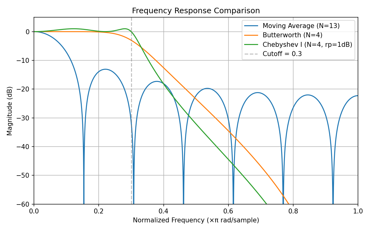
- The moving average filter (\(N=13\) ) already sits at \(-31.6\,\text{dB}\) at the nominal cutoff \(\text{Wn}=0.3\) , yet its first stopband sidelobe (near \(0.2205\pi\) ) peaks at only \(-13.09\,\text{dB}\) , with later sidelobes settling around \(-17\) to \(-22\,\text{dB}\) . The qualitative claim “shallow stopband attenuation” is backed by this measured \(-13\,\text{dB}\) figure.
- The Butterworth filter (\(N=4\)
) measures \(-3.014\,\text{dB}\)
exactly at \(\text{Wn}=0.3\)
, and the actual \(-3\,\text{dB}\)
crossing is at \(0.2999\pi\)
— confirming that
butter’sWnparameter literally means the \(-3\,\text{dB}\) point. - The Chebyshev Type I filter (\(N=4\)
, \(R_p=1\,\text{dB}\)
) measures only \(-1.005\,\text{dB}\)
(i.e. \(\approx -R_p\)
) at \(\text{Wn}=0.3\)
; its actual \(-3\,\text{dB}\)
crossing is at \(0.3135\pi\)
, wider than the Butterworth’s. In other words, specifying the same
Wn=0.3does not give the same \(-3\,\text{dB}\) bandwidth —cheby1’sWnmarks the passband-ripple edge, not \(-3\,\text{dB}\) , so its real \(-3\,\text{dB}\) bandwidth ends up roughly 4.5% wider than Butterworth’s (see the edge-case section below). At \(0.5\pi\) , Butterworth measures \(-23.45\,\text{dB}\) versus Chebyshev Type I’s \(-33.11\,\text{dB}\) — about \(10\,\text{dB}\) deeper at the same order, quantifying the sharper roll-off.
Reading the Group Delay
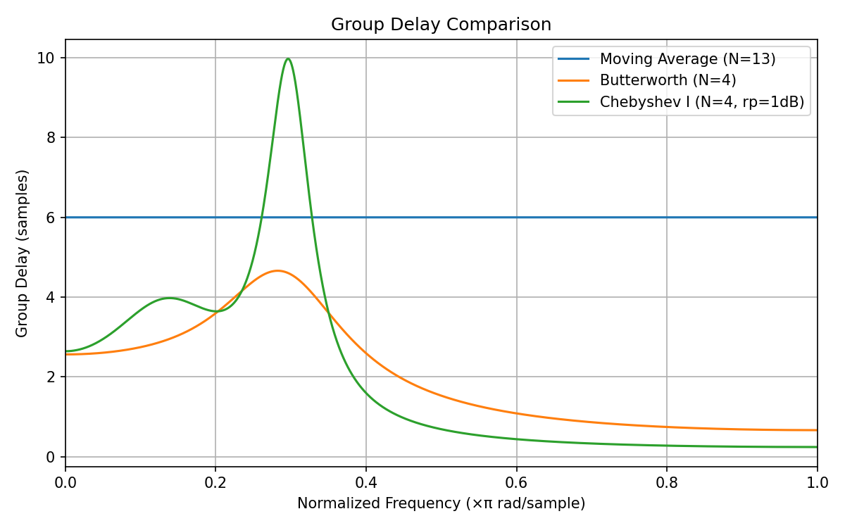
- The moving average filter has a constant group delay of \(6.000\) samples (\(=(N-1)/2=(13-1)/2\) ) at low frequency, at the cutoff (\(0.3\pi\) ), and at \(0.5\pi\) alike — numerically confirming perfectly linear phase.
- The Butterworth filter’s group delay is \(2.566\) samples at low frequency, peaks at \(4.567\) samples near the cutoff (\(0.3\pi\) ), then falls to \(1.528\) samples at \(0.5\pi\) .
- The Chebyshev Type I filter’s group delay peaks at \(9.870\) samples near the cutoff — more than double the Butterworth’s \(4.567\) samples under the same conditions. The equiripple design’s sharper transition band comes at the cost of markedly worse phase nonlinearity near the cutoff.
Reading the Step Response
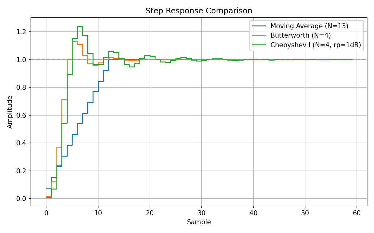
- The moving average filter reaches its steady-state value \(1.0000\) with \(0.00\%\) overshoot; its 2%-settling time is 12 samples.
- The Butterworth filter peaks at \(1.1322\) against a steady-state value of \(1.0000\) — an overshoot of \(13.22\%\) — and settles (2%) in 11 samples.
- The Chebyshev Type I filter peaks at \(1.1065\) , but its steady-state value is not \(1.0000\) — it is \(0.8915\) (\(\approx 10^{-1/20}=0.8913\) , the direct consequence of the even-order DC-gain edge case above). Measured against that steady-state value, the apparent overshoot balloons to \(24.12\%\) , and the 2%-settling time is 21 samples — the longest of the three.
What the Pole Locations Explain
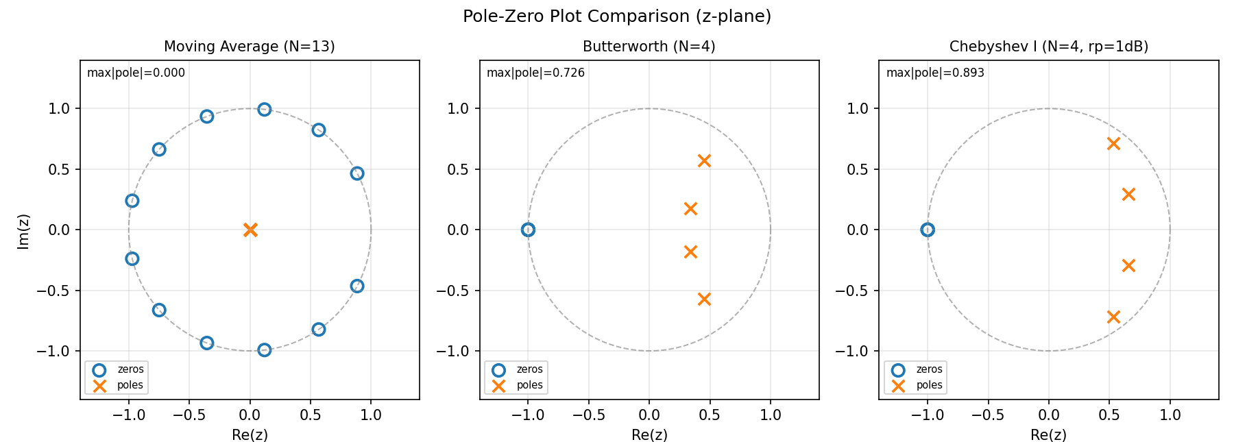
The pole-zero plot above (from tf2zpk) reveals the geometric reason behind these numbers.
- Moving average filter: since the denominator is constant (\(a=[1,0,\ldots,0]\)
), all 12 poles collapse onto the origin \(z=0\)
(
max|pole|=0.000) — an FIR filter. Having all poles at the origin is precisely what makes the group delay frequency-independent, i.e. linear phase. - Butterworth filter: the 4 poles sit at a maximum radius of \(0.726\) , roughly preserving the circular arrangement of equation \((7)\) after the bilinear transform to the z-plane.
- Chebyshev Type I filter: the 4 poles reach a maximum radius of \(0.893\) — closer to the unit circle than Butterworth’s. The elliptical arrangement of equation \((8)\) pushes poles closer to the unit circle, sharpening the transition band at the cost of lower damping — exactly matching the larger step-response overshoot, longer settling time, and higher group-delay peak measured above.
Filter Selection Guide
| Property | Moving Average | Butterworth | Chebyshev Type I |
|---|---|---|---|
| Passband | Flat | Maximally flat | Equiripple |
| Transition band | Gradual | Moderate | Sharp |
| Stopband attenuation | Shallow | Moderate | Deep |
| Phase | Linear | Nonlinear | Nonlinear |
| Group delay | Constant | Frequency-dependent | Frequency-dependent |
| Computational cost | Low | Moderate | Moderate |
| Primary use case | Noise smoothing | General-purpose filtering | Sharp cutoff required |
Guidelines for choosing a filter:
- When phase distortion must be avoided (waveform shape matters) — Moving average filter
- When passband flatness is critical (faithful reproduction of measurement signals) — Butterworth filter
- When the transition band must be as narrow as possible (separating adjacent frequency components) — Chebyshev Type I filter
Zero-Phase Filtering (filtfilt) Removes Group Delay
Butterworth and Chebyshev Type I are IIR filters with nonlinear phase, but for offline processing (post-processing recorded data), scipy.signal.filtfilt runs the signal forward and then backward through the same filter, canceling the apparent group delay. Because this is equivalent to applying the same filter twice, the frequency response gets squared.
import numpy as np
from scipy.signal import butter, cheby1, freqz, filtfilt

b_bw, a_bw = butter(4, 0.3)
b_cb, a_cb = cheby1(4, 1.0, 0.3)

w, h_bw = freqz(b_bw, a_bw, worN=8192)
w, h_cb = freqz(b_cb, a_cb, worN=8192)
freq = w / np.pi
idx_wn = np.argmin(np.abs(freq - 0.3))

# single-pass gain vs. the effective |H|^2 gain after filtfilt
mag_bw_single = 20 * np.log10(np.abs(h_bw[idx_wn]))
mag_bw_filtfilt = 20 * np.log10(np.abs(h_bw[idx_wn]) ** 2)
mag_cb_single = 20 * np.log10(np.abs(h_cb[idx_wn]))
mag_cb_filtfilt = 20 * np.log10(np.abs(h_cb[idx_wn]) ** 2)
print(f"Butterworth: single-pass {mag_bw_single:.3f} dB -> after filtfilt {mag_bw_filtfilt:.3f} dB")
print(f"Chebyshev I: single-pass {mag_cb_single:.3f} dB -> after filtfilt {mag_cb_filtfilt:.3f} dB")

# confirm zero delay via the peak location of the filtfilt impulse response
x = np.zeros(200)
x[100] = 1.0
y = filtfilt(b_bw, a_bw, x)
print("filtfilt impulse response peak index:", np.argmax(np.abs(y)), "(should be 100, matching the input peak)")
Output:
Butterworth: single-pass -3.014 dB -> after filtfilt -6.027 dB
Chebyshev I: single-pass -1.005 dB -> after filtfilt -2.011 dB
filtfilt impulse response peak index: 100 (should be 100, matching the input peak)
Because filtfilt passes the signal through the filter twice, the effective attenuation at the same nominal Wn exactly doubles in dB — Butterworth’s attenuation at cutoff goes from \(-3.014\,\text{dB}\)
to \(-6.027\,\text{dB}\)
, and Chebyshev Type I’s passband ripple expands from \(-1.005\,\text{dB}\)
to \(-2.011\,\text{dB}\)
. In other words, a filter meant for filtfilt should be designed slightly looser (lower order or a somewhat higher cutoff) than one intended for single-pass use, or it will end up narrower than intended. The impulse response peak, meanwhile, lands exactly on sample 100 — the same as the input — confirming the phase delay is completely eliminated.
Practical Edge Cases
The derivations and measurements above surface several pitfalls worth flagging explicitly.
The meaning of
Wndiffers between design functions:scipy.signal.butter’sWndenotes the \(-3\,\text{dB}\) point, whilescipy.signal.cheby1’sWndenotes the passband-ripple edge (\(-R_p\,\text{dB}\) ). As shown above, the sameWn=0.3yields an actual \(-3\,\text{dB}\) point of \(0.2999\pi\) for Butterworth versus \(0.3135\pi\) for Chebyshev Type I — assuming “same order and cutoff parameter means same bandwidth” leads to incorrect conclusions.The moving average filter’s stopband attenuation is inherently shallow: even its first sidelobe reaches only \(-13.09\,\text{dB}\) . If you need to reject a single interfering frequency, either tune \(N\) so a null lands exactly on it, or switch to a Savitzky-Golay filter or an IIR design.
An even-order Chebyshev Type I filter’s DC gain is not \(0\,\text{dB}\) : in our measurement (\(N=4\) , \(R_p=1\,\text{dB}\) ) the steady-state value is only \(0.8915\) , which can be a source of unexpected error in applications requiring faithful DC transmission.
High-order IIR filters can become numerically unstable in transfer-function (
b, a) form: not an issue at \(N=4\) , but risky at higher orders. Designingbutter(N, 0.3)at \(N=20,30,40,50\) and comparing the passband gain variation (over the first 400 bins, which should be perfectly flat) between theb,aform and thesos(second-order-sections) form gives:N=20: max|a|=3.258e+02 b,a passband deviation=2.103e-10 dB sos=2.604e-14 dB N=30: max|a|=1.186e+04 b,a passband deviation=3.248e-07 dB sos=3.857e-14 dB N=40: max|a|=4.462e+05 b,a passband deviation=1.295e-04 dB sos=4.436e-14 dB N=50: max|a|=1.745e+07 b,a passband deviation=2.441e-01 dB sos=4.436e-14 dBAt \(N=50\) , the denominator coefficients reach a magnitude of up to \(1.7\times10^7\) , and the
b,aform’s passband gain — which should be flat at \(0\,\text{dB}\) — deviates by up to \(0.24\,\text{dB}\) . Thesosform stays below \(10^{-14}\,\text{dB}\) of error under the same conditions, sooutput='sos'should be used once the order reaches double digits (no practical impact at the \(N=4\) order used in this article’s comparison).Two
scipy.signal.dlti/dsteppitfalls: (a)dlti/dsteprequirelen(a) >= len(b), so passing a pure-FIR filter like the moving average (\(a=[1.0]\) ) as-is raisesValueError: Improper transfer functionon recent SciPy (1.18.0 in this article’s verification environment) — zero-pad the denominator to match the numerator’s length. (b) The time arraytreturned bydstepis already 1-D, sot[0]is only its first (scalar) element, not the full time axis; for a single-input single-output system, plot againsttdirectly rather thant[0].flatten()(whileyremains a per-output tuple, soy[0].flatten()is correct). Both issues are already handled in the code above.
Recent Research: Cross-Family Comparisons of Heuristic, FIR, and IIR Filters on Real Data
The approach in this article — comparing distinct filter families under matched conditions — also appears in empirical validation studies. Raju, Friedman, Bouman, and Komogortsev (2023) applied heuristic moving-average-style filters (STD/EXTRA), a Savitzky-Golay filter, an IIR (Butterworth) filter, and an FIR filter to eye-movement data recorded with an EyeLink 1000 eye tracker, and quantitatively compared their noise-removal performance (Journal of Eye Movement Research, 2023).
They report that the frequency reaching \(-30\,\text{dB}\)
attenuation was \(93\,\text{Hz}\)
for the FIR filter, \(102\,\text{Hz}\)
for the IIR (Butterworth) filter, and \(204\,\text{Hz}\)
for the Savitzky-Golay filter — showing the FIR and IIR designs achieve much sharper transition bands than the heuristic filter. Velocity-signal noise (standard deviation) fell from \(120.19\,\text{deg/s}\)
unfiltered to roughly \(23\,\text{deg/s}\)
for both FIR and IIR. Both the FIR and IIR filters were implemented with bidirectional (zero-phase) filtering — the same idea covered in this article’s filtfilt section — to eliminate phase delay. On the downside, they also report that every digital filter increased the signal’s lag-1 autocorrelation from \(0.58\)
(unfiltered) to roughly \(0.97\)
, a reminder that noise removal changes the time series’ statistical structure (autocorrelation) — a side effect that is easy to overlook when choosing a filter.
This finding reinforces, with real-world data rather than theory alone, the same pattern this article demonstrates: the moving average (a degenerate FIR design), Butterworth (IIR), and Chebyshev Type I (IIR) share the property that FIR/IIR designs achieve sharper transition bands and stronger noise suppression than heuristic smoothing.
Conclusion
This article presented the theoretical background for three low-pass filters — moving average, Butterworth, and Chebyshev Type I — deriving each magnitude response (maximal flatness / equiripple) and pole location, then measured their frequency response, group delay, step response, and pole-zero placement under matched order and cutoff conditions in Python.
The key measured findings are:
- The same
Wnmeans different things across design functions:butter’sWnis the \(-3\,\text{dB}\) point, whilecheby1’s is the passband-ripple edge, so Chebyshev Type I’s true \(-3\,\text{dB}\) bandwidth ends up roughly 4.5% wider (measured: \(0.2999\pi\) for Butterworth vs. \(0.3135\pi\) for Chebyshev Type I). - The moving average filter’s first stopband sidelobe reaches only \(-13.09\,\text{dB}\) — its stopband attenuation is inherently shallow.
- The even-order Chebyshev Type I filter’s step response settles at \(0.8915\) , not \(1.0\) , inflating its apparent overshoot to \(24.12\%\) .
- In the pole-zero plot, Chebyshev Type I’s maximum pole radius (\(0.893\) ) sits closer to the unit circle than Butterworth’s (\(0.726\) ) — the geometric root cause of its larger group-delay peak (\(9.870\) vs. \(4.567\) samples) and larger overshoot.
Each filter has its own strengths and weaknesses; choosing the right one depends on the requirements of the application. For related material on the EMA filter (a first-order IIR filter), see also Frequency Characteristics of the Exponential Moving Average Filter . For a systematic overview of state-space model-based filtering methods (Kalman filter, EKF, UKF, particle filter), see Fundamentals of Filtering Methods in Signal Processing .
Related Articles
- Frequency Characteristics of the EMA Filter - Derives the EMA transfer function and analyzes its frequency response.
- Moving Average Filters Compared: SMA, WMA, and EMA in Python - Compares the types and characteristics of moving average filters.
- Fast Fourier Transform (FFT): Theory and Python Implementation - Covers FFT fundamentals used for frequency response analysis.
- Fundamentals of Filtering Methods in Signal Processing - Systematic overview of Kalman filter, EKF, UKF, and particle filter.
- Butterworth Filter Design: Theory and Python Implementation - Detailed coverage of Butterworth filter mathematical foundations and implementation.
- FIR vs IIR Filters: Characteristics, Design, and Python Implementation - Compares phase characteristics and stability of moving average (FIR) and Butterworth (IIR) filters.
- Wiener Filter: Optimal Linear Filtering Theory and Python Implementation - Covers optimal filter design based on SNR.
- Notch Filter Design and Python Implementation - Explains notch filter design for removing specific frequencies.
- Savitzky-Golay Filter: Theory and Python Implementation - An evolution of the moving average that preserves signal shape through polynomial fitting.
- Chebyshev Filter Design: Theory and Python Implementation - Detailed design and characteristics of Type I/II equiripple IIR filters.
- Bessel Filter: Theory and Python Implementation - IIR filter design that maximizes flat group delay.
- Elliptic (Cauer) Filter: Theory and Python Implementation - IIR filter that achieves the steepest transition band for a given order.
- Bandpass Filter Design: Theory and Python Implementation - Combine an LPF with an HPF to form a bandpass — the natural next step after lowpass design.
- Adaptive Filters (LMS/RLS): Theory and Python Implementation - In contrast to fixed lowpass designs, adaptive filters update their coefficients automatically based on signal statistics.
- Filter Design Selection Guide: 3 axes and characteristic comparison — Use this hub to position the lowpass family against alternatives during selection.
References
- A. V. Oppenheim, R. W. Schafer, “Discrete-Time Signal Processing,” Prentice Hall.
- scipy.signal — Signal processing (SciPy documentation)
- Raju, M. H., Friedman, L., Bouman, T. M., & Komogortsev, O. V. (2023). “Filtering Eye-Tracking Data From an EyeLink 1000: Comparing Heuristic, Savitzky-Golay, IIR and FIR Digital Filters.” Journal of Eye Movement Research, 16(3). PMC11219126