What is a Particle Filter?
The particle filter (also known as the Sequential Monte Carlo method, SMC) is a nonlinear filtering technique that represents the posterior distribution of the state using a set of weighted samples called particles. Unlike Gaussian-approximation filters, it requires no distributional assumptions and can handle arbitrary nonlinear and non-Gaussian systems.
Gaussian-approximation filters such as the Cubature Kalman Filter (CKF) and the Unscented Transform -based Unscented Kalman Filter (UKF) degrade in accuracy when the posterior distribution is multimodal or the system exhibits strong nonlinearities. The particle filter remains effective in these situations.
The particle filter shares its Monte Carlo sampling foundation with the Cross-Entropy Method (CEM) , but whereas CEM targets optimization problems, the particle filter targets sequential state estimation in time series.
Algorithm Overview
State-Space Model
Consider the following nonlinear state-space model:
\[ x_k = f(x_{k-1}) + w_{k-1}, \quad w_{k-1} \sim p_w \] \[ y_k = h(x_k) + v_k, \quad v_k \sim p_v \]where \(f\) is the state transition function, \(h\) is the observation function, and \(w_{k-1}\) , \(v_k\) are the process and observation noise respectively. The noise distributions \(p_w, p_v\) need not be Gaussian.
Sequential Monte Carlo Framework
The particle filter approximates the posterior distribution \(p(x_k | y_{1:k})\) using \(N\) weighted particles \(\{x_k^{(i)}, w_k^{(i)}\}_{i=1}^{N}\) . Each step consists of three phases.
1. Prediction: Propagate each particle through the state transition model:
\[ x_k^{(i)} \sim p(x_k | x_{k-1}^{(i)}) \]In practice, this is implemented as \(x_k^{(i)} = f(x_{k-1}^{(i)}) + w_{k-1}^{(i)}\) by adding process noise.
2. Weight Update: Compute the likelihood of the new observation \(y_k\) for each particle and update the weights:
\[ w_k^{(i)} \propto p(y_k | x_k^{(i)}) \]3. Normalization: Normalize the weights so they sum to one:
\[ \tilde{w}_k^{(i)} = \frac{w_k^{(i)}}{\sum_{j=1}^{N} w_k^{(j)}} \]The state estimate is then computed as a weighted average:
\[ \hat{x}_k = \sum_{i=1}^{N} \tilde{w}_k^{(i)} x_k^{(i)} \]Derivation from Importance Sampling
The weight update rule from the previous section, \(w_k^{(i)} \propto p(y_k \mid x_k^{(i)})\) , may look like it was pulled out of thin air. In fact, it is a simplification of the general Sequential Importance Sampling (SIS) update for a specific choice of proposal distribution. Here we derive it from first principles.
The Importance Sampling Principle
When we cannot sample directly from the target distribution \(p(x_{0:k} \mid y_{1:k})\) , we instead draw particles \(x_{0:k}^{(i)} \sim q\) from a proposal distribution \(q(x_{0:k} \mid y_{1:k})\) and correct for the mismatch using importance weights:
\[ w_k^{(i)} \propto \frac{p(x_{0:k}^{(i)} \mid y_{1:k})}{q(x_{0:k}^{(i)} \mid y_{1:k})} \]The expectation of any function \(g\) can then be approximated by the self-normalized importance sampling estimator:
\[ \mathbb{E}[g(x_k) \mid y_{1:k}] \approx \sum_{i=1}^{N} \tilde{w}_k^{(i)} g(x_k^{(i)}) \]The catch is that the dimensionality of the full trajectory \(x_{0:k}\) grows with \(k\) , so recomputing the weight from scratch at every step would make the cost grow without bound over time.
Reducing to a Recursion
Factorize the proposal distribution using the Markov property:
\[ q(x_{0:k} \mid y_{1:k}) = q(x_0) \prod_{t=1}^{k} q(x_t \mid x_{0:t-1}, y_{1:t}) \]The target distribution factorizes similarly, from the Markov property of the state-space model and Bayes’ rule:
\[ p(x_{0:k} \mid y_{1:k}) \propto p(x_0) \prod_{t=1}^{k} p(y_t \mid x_t) \, p(x_t \mid x_{t-1}) \](Proof: \(p(x_{0:k}, y_{1:k}) = p(x_0) \prod_t p(x_t \mid x_{t-1}) p(y_t \mid x_t)\) is exactly the generative process of the state-space model, and \(p(x_{0:k} \mid y_{1:k}) \propto p(x_{0:k}, y_{1:k})\) follows directly.)
Taking the ratio of the two factorizations, the weight reduces to the previous time step’s weight multiplied by a single new factor — a recursive update:
\[ w_k^{(i)} \propto w_{k-1}^{(i)} \cdot \frac{p(y_k \mid x_k^{(i)}) \, p(x_k^{(i)} \mid x_{k-1}^{(i)})}{q(x_k^{(i)} \mid x_{k-1}^{(i)}, y_k)} \]This is the general SIS update. Because it only requires the previous weight \(w_{k-1}^{(i)}\) and the new particle \(x_k^{(i)}\) — not the full trajectory \(x_{0:k-1}\) — the computation stays sequential.
Specializing to the Bootstrap Filter
If we choose the proposal to be the state transition model itself, \(q(x_k \mid x_{k-1}, y_k) = p(x_k \mid x_{k-1})\) (i.e., particles are propagated while ignoring the new observation \(y_k\) ), the \(p(x_k \mid x_{k-1})\) terms in the numerator and denominator cancel, leaving
\[ w_k^{(i)} \propto w_{k-1}^{(i)} \cdot p(y_k \mid x_k^{(i)}) \]Immediately after resampling, \(w_{k-1}^{(i)} = 1/N\) for all particles, so this reduces to the formula from the previous section, \(w_k^{(i)} \propto p(y_k \mid x_k^{(i)})\) . This special case is called the bootstrap filter (Gordon, Salmond & Smith, 1993). It is the simplest to implement, but since the proposal ignores the observation entirely, it tends to produce high-variance weights whenever the likelihood \(p(y_k \mid x_k)\) is sharply peaked (i.e., when observation noise is small). The code implementation in this article is a bootstrap filter.
Effective Sample Size and Degeneracy
A major challenge in particle filtering is weight degeneracy: over time, most particles acquire negligibly small weights while a few particles dominate. This degeneracy is quantified by the Effective Sample Size (ESS):
\[ N_{\text{eff}} = \frac{1}{\sum_{i=1}^{N} (\tilde{w}_k^{(i)})^2} \]\(N_{\text{eff}}\) ranges from 1 to \(N\) . When all weights are equal (no degeneracy), \(N_{\text{eff}} = N\) . Resampling is triggered when \(N_{\text{eff}}\) drops below a threshold, typically \(N/2\) .
Deriving the Effective Sample Size
This formula, too, might look arbitrary, but it can be derived from an approximation due to Kong, Liu & Wong (1994). Ideally, we would like to measure how much the variance of the self-normalized importance sampling estimator degrades relative to the variance we would get from \(N\) i.i.d. draws directly from the target distribution. They showed that this degradation factor can be approximated using the squared coefficient of variation of the unnormalized importance ratio \(r^{(i)} = p(x^{(i)})/q(x^{(i)})\) :
\[ \mathrm{CV}^2(w) = \frac{\mathrm{Var}(r)}{\mathbb{E}[r]^2} \]as \(1 + \mathrm{CV}^2(w)\) . The effective sample size is then defined as
\[ N_{\text{eff}} \approx \frac{N}{1 + \mathrm{CV}^2(w)} \]Using the normalized weights \(\tilde{w}^{(i)}\) (with \(\sum_i \tilde{w}^{(i)} = 1\) ), whose sample mean is \(1/N\) , \(\mathrm{CV}^2(w)\) can be rewritten as:
\[ \mathrm{CV}^2(w) = N^2 \cdot \frac{1}{N} \sum_{i=1}^{N} \left(\tilde{w}^{(i)} - \frac{1}{N}\right)^2 = N \sum_{i=1}^{N} (\tilde{w}^{(i)})^2 - 1 \](using \(\sum_i \tilde{w}^{(i)} = 1\) in the expansion). Substituting back into the \(N_{\text{eff}}\) formula gives
\[ N_{\text{eff}} \approx \frac{N}{1 + \left(N \sum_i (\tilde{w}^{(i)})^2 - 1\right)} = \frac{N}{N \sum_i (\tilde{w}^{(i)})^2} = \frac{1}{\sum_{i=1}^{N} (\tilde{w}^{(i)})^2} \]which recovers the formula used in the code. When all particles have equal weight (\(\tilde{w}^{(i)} = 1/N\) ), \(\mathrm{CV}^2 = 0\) and \(N_{\text{eff}} = N\) ; when the weight collapses onto a single particle (all others zero), \(\mathrm{CV}^2 \to N-1\) and \(N_{\text{eff}} \to 1\) — matching intuition.
def effective_sample_size(weights):
    """Compute the effective sample size."""
    return 1.0 / np.sum(weights ** 2)
Why Resampling Is Necessary: A Proof of Weight Variance Growth
The weight update from the previous section, \(w_k^{(i)} \propto w_{k-1}^{(i)} \cdot p(y_k \mid x_k^{(i)}) p(x_k^{(i)} \mid x_{k-1}^{(i)}) / q(\cdot)\) , is a multiplicative recursion. As long as the new factor introduced at each time step varies across particles (which holds in general unless the proposal \(q\) exactly matches the target), \(\log w_k^{(i)}\) behaves like a random walk that accumulates independent random fluctuations at every step. Consequently, \(\mathrm{Var}(w_k)\) is non-decreasing in time, and without resampling, the weight variance diverges as \(k \to \infty\) , with \(N_{\text{eff}} \to 1\) (proven rigorously by Doucet, Godsill & Andrieu, 2000). Resampling counteracts this by resetting all weights to be equal whenever \(N_{\text{eff}}\) drops below the threshold, periodically restarting this random walk and preventing the variance from diverging. This is the formal justification for why resampling is necessary.
Resampling Methods
Resampling reconstructs the particle set by duplicating high-weight particles and discarding low-weight ones. Below are three widely used methods, plus a naive baseline for comparison.
Systematic Resampling
Systematic resampling generates a single random number \(u_0\) and places equally spaced points along the cumulative distribution function (CDF). It has \(O(N)\) complexity and low variance, making it the most commonly used method in practice.
def systematic_resampling(weights):
    """Systematic resampling."""
    N = len(weights)
    positions = (np.random.random() + np.arange(N)) / N
    cumsum = np.cumsum(weights)
    indices = np.zeros(N, dtype=int)
    i, j = 0, 0
    while i < N:
        if positions[i] < cumsum[j]:
            indices[i] = j
            i += 1
        else:
            j += 1
    return indices
Residual Resampling
Residual resampling first deterministically copies each particle \(\lfloor N \tilde{w}^{(i)} \rfloor\) times, then samples the remaining particles probabilistically from the residual weights. The deterministic component reduces variance compared to purely random methods.
def residual_resampling(weights):
    """Residual resampling."""
    N = len(weights)
    indices = []

    # Deterministic copies
    num_copies = (N * weights).astype(int)
    for i in range(N):
        indices.extend([i] * num_copies[i])

    # Handle residuals
    residual_weights = N * weights - num_copies
    residual_weights /= residual_weights.sum()
    num_remaining = N - len(indices)
    if num_remaining > 0:
        cumsum = np.cumsum(residual_weights)
        # Apply systematic resampling to the residual part
        positions = (np.random.random() + np.arange(num_remaining)) / num_remaining
        i, j = 0, 0
        while i < num_remaining:
            if positions[i] < cumsum[j]:
                indices.append(j)
                i += 1
            else:
                j += 1

    return np.array(indices)
Stratified Resampling
Stratified resampling divides the \([0, 1)\) interval into \(N\) equal strata and draws an independent uniform random number within each stratum to sample from the CDF. It is similar to systematic resampling but uses independent random numbers per stratum.
def stratified_resampling(weights):
    """Stratified resampling."""
    N = len(weights)
    positions = (np.random.random(N) + np.arange(N)) / N
    cumsum = np.cumsum(weights)
    indices = np.zeros(N, dtype=int)
    i, j = 0, 0
    while i < N:
        if positions[i] < cumsum[j]:
            indices[i] = j
            i += 1
        else:
            j += 1
    return indices
Multinomial Resampling (Baseline) and the Theory of Offspring-Count Variance
To quantify how much the three methods above actually reduce variance, we need a baseline for comparison. Multinomial resampling is the most naive approach: it draws \(N\) indices independently from the categorical distribution defined by the normalized weights.
def multinomial_resampling(weights):
    """Multinomial resampling (naive baseline)."""
    N = len(weights)
    return np.random.choice(N, size=N, replace=True, p=weights)
Deriving the offspring-count variance: Let \(N_i\) denote the number of times particle \(i\) is duplicated (the “offspring count”, with \(\sum_i N_i = N\) ). Every unbiased resampling scheme satisfies \(\mathbb{E}[N_i] = N \tilde{w}^{(i)}\) , but \(\mathrm{Var}(N_i)\) differs sharply between methods.
Under multinomial resampling, \(N_i\) is the number of times particle \(i\) is chosen out of \(N\) independent trials, so \(N_i \sim \mathrm{Binomial}(N, \tilde{w}^{(i)})\) , giving
\[ \mathrm{Var}(N_i) = N \tilde{w}^{(i)} (1 - \tilde{w}^{(i)}) \]which is maximized at \(\tilde{w}^{(i)} = 1/2\) , reaching \(N/4\) — a value that can grow proportionally with \(N\) .
By contrast, systematic and stratified resampling place equally spaced (or per-stratum) points on the CDF, so the number of points landing inside particle \(i\) ’s cumulative interval (width \(\tilde{w}^{(i)}\) ) can only take one of two adjacent integer values: \(\lfloor N \tilde{w}^{(i)} \rfloor\) or \(\lceil N \tilde{w}^{(i)} \rceil\) . A random variable restricted to two values has variance at most \(1/4\) (the upper bound for a Bernoulli-type variable), so
\[ \mathrm{Var}(N_i) \le \frac{1}{4} \]holds regardless of \(\tilde{w}^{(i)}\) — a constant bound independent of \(N\) , unlike multinomial resampling’s \(N \tilde{w}^{(i)}(1-\tilde{w}^{(i)})\) , which grows with \(N\) (Douc & Cappe, 2005). Residual resampling deterministically copies the integer part and applies systematic resampling only to the residual, so its variance ends up at roughly the same level as systematic resampling.
Empirical verification: We ran all four methods 20,000 times each on a skewed weight vector (\(N=200\) , drawn from the square of an exponential distribution) and measured the empirical variance of each particle’s offspring count.
np.random.seed(0)
N = 200
raw = np.random.exponential(scale=1.0, size=N) ** 2
weights_fixed = raw / raw.sum()

n_trials = 20000
for name, fn in resamplers.items():
    counts = np.zeros((n_trials, N))
    for t in range(n_trials):
        idx = fn(weights_fixed)
        counts[t] = np.bincount(idx, minlength=N)
    print(f"{name}: mean Var(N_i)={counts.var(axis=0).mean():.4f}, "
          f"max Var(N_i)={counts.var(axis=0).max():.4f}")
The results matched the theory with high precision:
| Method | Mean Var(\(N_i\) ) | Max Var(\(N_i\) ) | Total \(\sum_i\) Var(\(N_i\) ) | Ratio to Multinomial |
|---|---|---|---|---|
| Multinomial (baseline) | 0.9685 | 21.0489 | 194.22 | 100% |
| Systematic | 0.1334 | 0.2499 | 26.64 | 13.7% |
| Residual | 0.1335 | 0.2498 | 26.69 | 13.7% |
| Stratified | 0.1891 | 0.4968 | 37.83 | 19.5% |
The theoretical values (mean binomial variance 0.9692, max 21.0006) closely match the empirical results, and the empirical maxima for systematic and residual resampling (0.2499, 0.2498) agree with the theoretical upper bound \(1/4 = 0.25\) . The total variance of systematic and residual resampling is only 13.7% that of multinomial resampling, numerically confirming the variance-reduction effect proven theoretically by Douc & Cappe (2005). Stratified resampling draws one independent random number per stratum (\(N\) total), so it has more sources of randomness than systematic resampling (a single draw), which is reflected in its somewhat higher variance (19.5%).
| Property | Systematic | Residual | Stratified | Multinomial (baseline) |
|---|---|---|---|---|
| Complexity | O(N) | O(N) | O(N) | O(N) |
| Variance | Low (13.7% of mult.) | Lowest (13.7% of mult.) | Low (19.5% of mult.) | Highest (100%, baseline) |
| Random draws | 1 | Remaining only | N | N |
| Deterministic component | No | Yes (floor copies) | No | No |
Nonlinear System Demo
Benchmark Model
To evaluate particle filter performance, we use the widely adopted Univariate Nonstationary Growth Model. This model exhibits strong nonlinearity that challenges Gaussian-approximation filters.
State transition model:
\[ x_k = \frac{x_{k-1}}{2} + \frac{25 x_{k-1}}{1 + x_{k-1}^2} + 8\cos(1.2k) + w_k, \quad w_k \sim \mathcal{N}(0, \sigma_w^2) \]Observation model:
\[ y_k = \frac{x_k^2}{20} + v_k, \quad v_k \sim \mathcal{N}(0, \sigma_v^2) \]A key feature of this model is that the observation function \(h(x) = x^2/20\) is an even function, so positive and negative state values are indistinguishable from observations alone. This can produce a bimodal posterior distribution.
Particle Filter Implementation
import numpy as np
import matplotlib.pyplot as plt

# ---- Model definition ----
sigma_w = np.sqrt(10.0)  # process noise std
sigma_v = np.sqrt(1.0)   # observation noise std

def state_transition(x, k):
    """State transition function."""
    return x / 2.0 + 25.0 * x / (1.0 + x ** 2) + 8.0 * np.cos(1.2 * k)

def observation(x):
    """Observation function."""
    return x ** 2 / 20.0

def log_likelihood(y, x):
    """Log-likelihood log p(y|x)."""
    diff = y - observation(x)
    return -0.5 * (diff ** 2) / (sigma_v ** 2)

# ---- Particle filter ----
def particle_filter(y_obs, N_particles, resample_fn, resample_threshold=0.5):
    """
    Run the particle filter.

    Parameters
    ----------
    y_obs : array, observation sequence
    N_particles : int, number of particles
    resample_fn : callable, resampling function
    resample_threshold : float, ESS threshold (ratio of N_particles)

    Returns
    -------
    x_est : array, state estimate sequence
    ess_history : array, ESS history
    """
    T = len(y_obs)
    threshold = resample_threshold * N_particles

    # Initialize: sample from prior
    particles = np.random.normal(0, np.sqrt(5.0), N_particles)
    weights = np.ones(N_particles) / N_particles

    x_est = np.zeros(T)
    ess_history = np.zeros(T)

    for k in range(T):
        # Prediction: state transition + process noise
        particles = state_transition(particles, k + 1) \
                    + sigma_w * np.random.randn(N_particles)

        # Weight update: compute in log domain for numerical stability
        log_w = log_likelihood(y_obs[k], particles)
        log_w -= np.max(log_w)  # numerical stabilization
        weights = np.exp(log_w)
        weights /= np.sum(weights)

        # State estimate
        x_est[k] = np.sum(weights * particles)

        # ESS computation
        ess = effective_sample_size(weights)
        ess_history[k] = ess

        # Resampling (ESS threshold-based)
        if ess < threshold:
            indices = resample_fn(weights)
            particles = particles[indices]
            weights = np.ones(N_particles) / N_particles

    return x_est, ess_history
Running the Simulation
np.random.seed(42)
T = 100            # number of time steps
N_particles = 500  # number of particles

# Generate true state and observations
x_true = np.zeros(T)
y_obs = np.zeros(T)
x_true[0] = 0.1  # initial state

for k in range(1, T):
    x_true[k] = state_transition(x_true[k - 1], k) \
                + sigma_w * np.random.randn()

for k in range(T):
    y_obs[k] = observation(x_true[k]) + sigma_v * np.random.randn()

# Run particle filter with three resampling methods + a comparison baseline
resamplers = {
    "Systematic": systematic_resampling,
    "Residual": residual_resampling,
    "Stratified": stratified_resampling,
    "Multinomial": multinomial_resampling,
}

results = {}
for name, fn in resamplers.items():
    np.random.seed(42)  # same seed for fair comparison
    x_est, ess_hist = particle_filter(y_obs, N_particles, fn)
    rmse = np.sqrt(np.mean((x_true - x_est) ** 2))
    results[name] = {"estimate": x_est, "ess": ess_hist, "rmse": rmse}
    print(f"{name}: RMSE = {rmse:.4f}")
Visualization
fig, axes = plt.subplots(2, 1, figsize=(12, 8), sharex=True)

# State estimation comparison
axes[0].plot(x_true, "k-", linewidth=1.5, label="True state")
colors = {"Systematic": "#2a78d6", "Residual": "#1baf7a",
          "Stratified": "#eda100", "Multinomial": "#e34948"}
for name, res in results.items():
    axes[0].plot(res["estimate"], "--", color=colors[name],
                 linewidth=1, label=f"{name} (RMSE={res['rmse']:.2f})")
axes[0].set_ylabel("State $x_k$")
axes[0].set_title("Particle Filter: Resampling Method Comparison")
axes[0].legend(loc="upper right", fontsize=9)
axes[0].grid(True, alpha=0.3)

# ESS over time
for name, res in results.items():
    axes[1].plot(res["ess"], color=colors[name], linewidth=0.8, label=name)
axes[1].axhline(y=N_particles / 2, color="red", linestyle=":",
                label=f"Threshold (N/2={N_particles // 2})")
axes[1].set_xlabel("Time step $k$")
axes[1].set_ylabel("Effective Sample Size")
axes[1].legend(loc="upper right", fontsize=9)
axes[1].grid(True, alpha=0.3)

plt.tight_layout()
plt.savefig("particle_filter_comparison.png", dpi=150)
plt.show()
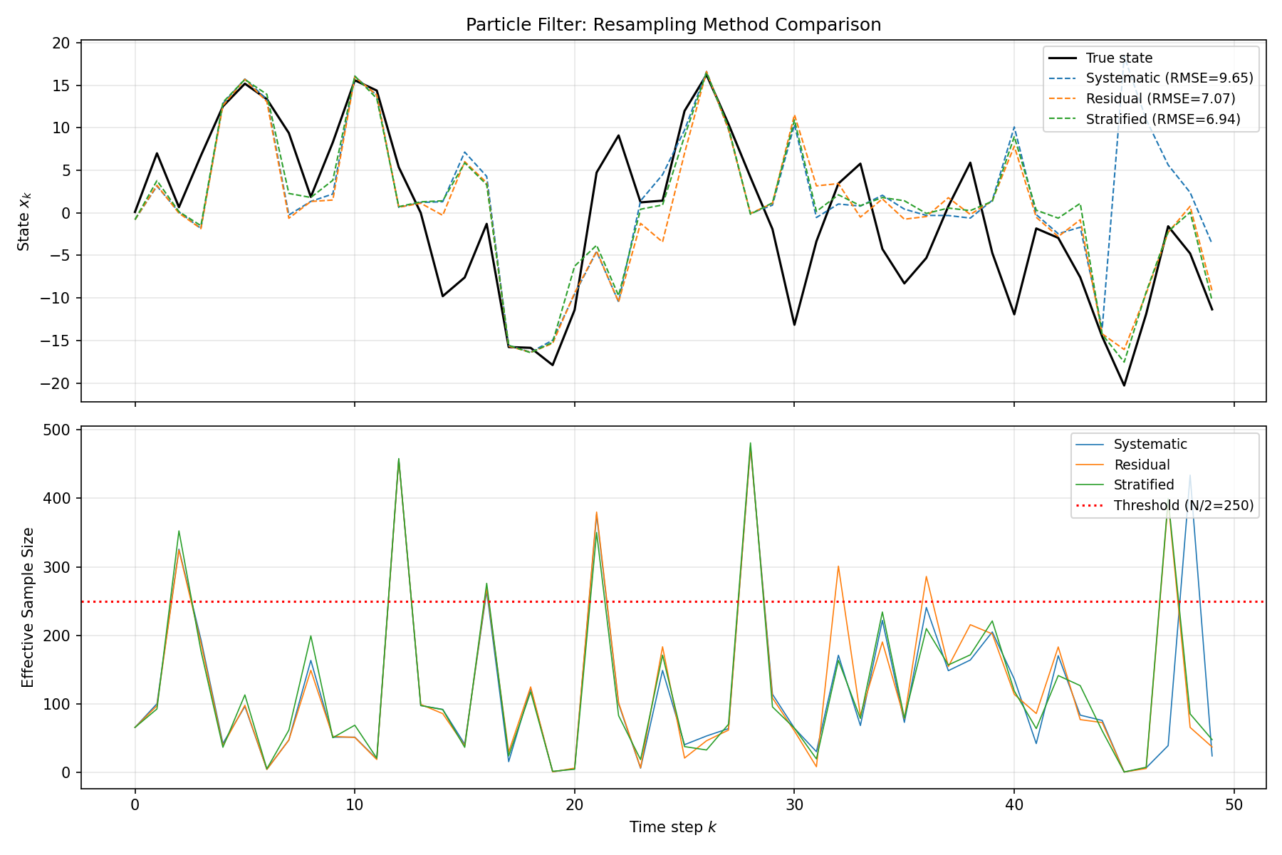
Running the Code and Checking Robustness
Actually running the code above (with np.random.seed(42) fixed, \(T=100\)
, \(N=500\)
) gives the following RMSE values:
- Systematic: RMSE = 7.5868
- Residual: RMSE = 7.6643
- Stratified: RMSE = 7.2864
- Multinomial: RMSE = 7.4957
Looking only at this single run, the naive multinomial resampling actually beats systematic and residual resampling on RMSE — which might seem to contradict the previous section’s theory that multinomial resampling has strictly worse offspring-count variance. But this is the result of a single seed (one true state trajectory, one random stream), which is not enough to draw a statistical conclusion. So we generated 100 independent true-state/observation sequences and ran all four methods on each.
n_mc = 100
mc_rmse = {name: np.zeros(n_mc) for name in resamplers}
mc_mean_ess = {name: np.zeros(n_mc) for name in resamplers}
master_seed = np.random.SeedSequence(2026)
child_seeds = master_seed.spawn(n_mc)

for trial in range(n_mc):
    rng = np.random.default_rng(child_seeds[trial])
    xt = np.zeros(T)
    yo = np.zeros(T)
    xt[0] = 0.1
    for k in range(1, T):
        xt[k] = state_transition(xt[k - 1], k) + sigma_w * rng.standard_normal()
    for k in range(T):
        yo[k] = observation(xt[k]) + sigma_v * rng.standard_normal()

    for name, fn in resamplers.items():
        np.random.seed(int(child_seeds[trial].generate_state(1)[0]) ^ hash(name) % (2**31))
        x_est, ess_hist = particle_filter(yo, N_particles, fn)[:2]
        mc_rmse[name][trial] = np.sqrt(np.mean((xt - x_est) ** 2))
        mc_mean_ess[name][trial] = ess_hist.mean()

for name in resamplers:
    r, e = mc_rmse[name], mc_mean_ess[name]
    print(f"{name}: RMSE mean={r.mean():.4f} std={r.std():.4f} mean ESS={e.mean():.2f}")
The results from 100 independent trials:
| Method | RMSE mean | RMSE std | Mean ESS |
|---|---|---|---|
| Systematic | 10.5868 | 1.3849 | 118.89 |
| Residual | 10.5706 | 1.3136 | 118.67 |
| Stratified | 10.5685 | 1.3886 | 118.95 |
| Multinomial | 10.4065 | 1.3415 | 119.61 |
The differences in mean RMSE across the four methods (at most about 0.18) are tiny compared to the trial-to-trial standard deviation (about 1.3–1.4). In other words, under this nonlinear growth model with \(N=500\) , despite the theoretical difference in offspring-count variance (13.7%–100%), the overall impact on filtering error is small enough to be swamped by trial-to-trial variability from process and observation noise. This does not mean the choice of resampling method is unimportant in general — rather, it suggests that (1) when process noise is large enough, as in this model (\(\sigma_w = \sqrt{10}\) ), particle diversity is regenerated every step and the differences between methods shrink accordingly, and (2) the differences matter most under the low-noise, high-dimensional, long-horizon conditions discussed in the next section, where sample impoverishment becomes severe.
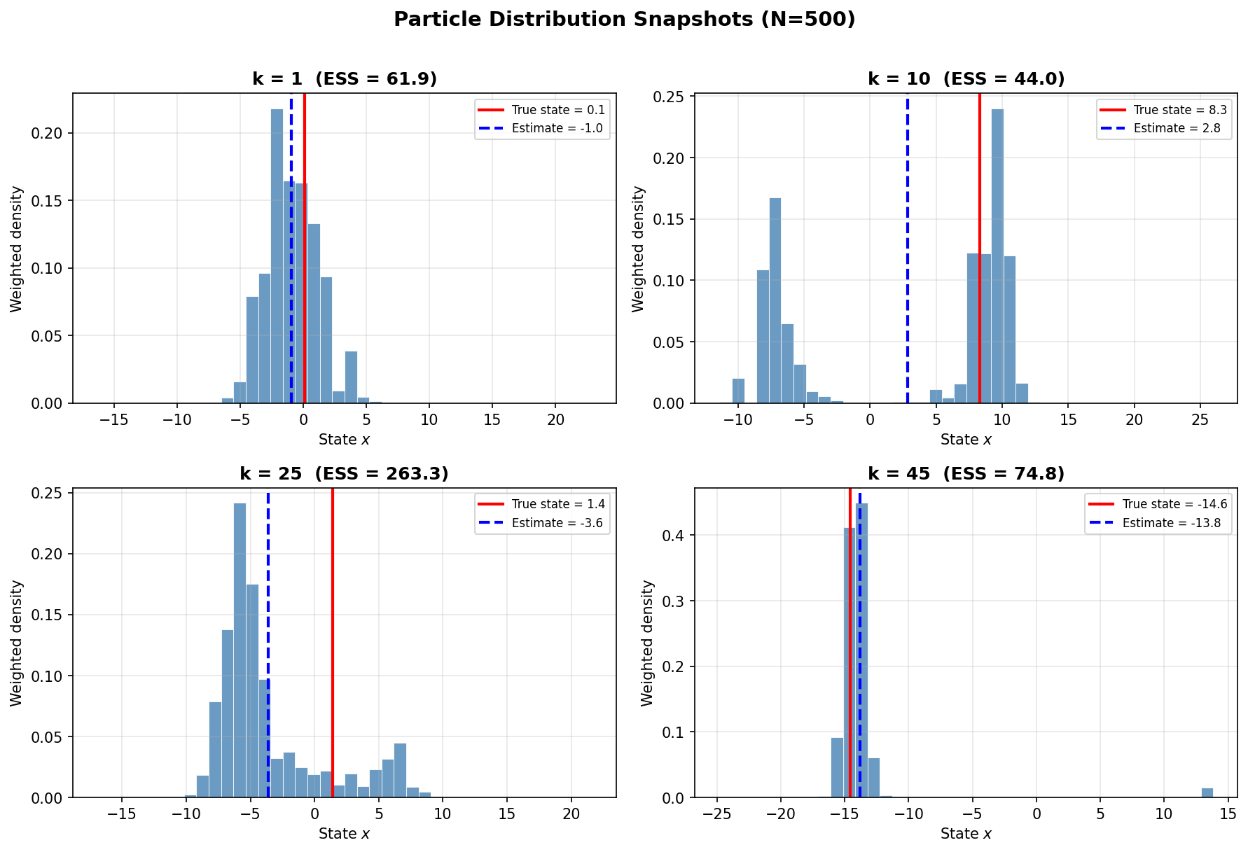
Particle Distribution Snapshots
The figure below shows the weighted particle distribution (histogram) at selected time steps. The red line indicates the true state, and the blue line shows the estimate.
Edge Cases and Practical Pitfalls
Sample Impoverishment
Resampling fixes weight degeneracy, but it introduces a new failure mode. Because it duplicates high-weight particles and discards low-weight ones, the number of distinct values in the particle set right after resampling is bounded above by the pre-resampling \(N_{\text{eff}}\) . Unless the process noise at the next prediction step regenerates enough diversity, this shrinkage of the number of unique ancestors compounds across resampling events, and the particle cloud eventually collapses onto a single value. This is called sample impoverishment (or path degeneracy). It is especially fatal for problems with small process noise, or for static parameter estimation (where process noise is effectively zero) — which is precisely why particle filters alone are unsuited to static parameter estimation (Particle MCMC and SMC² are among the methods proposed to address this).
Measuring how often resampling was triggered and the average fraction of unique particles surviving each resampling event in this article’s simulation (\(T=100\) , \(N=500\) ) gives:
| Method | Resampling events | Mean unique-particle fraction |
|---|---|---|
| Systematic | 85 | 0.220 |
| Residual | 87 | 0.222 |
| Stratified | 87 | 0.220 |
| Multinomial | 85 | 0.194 |
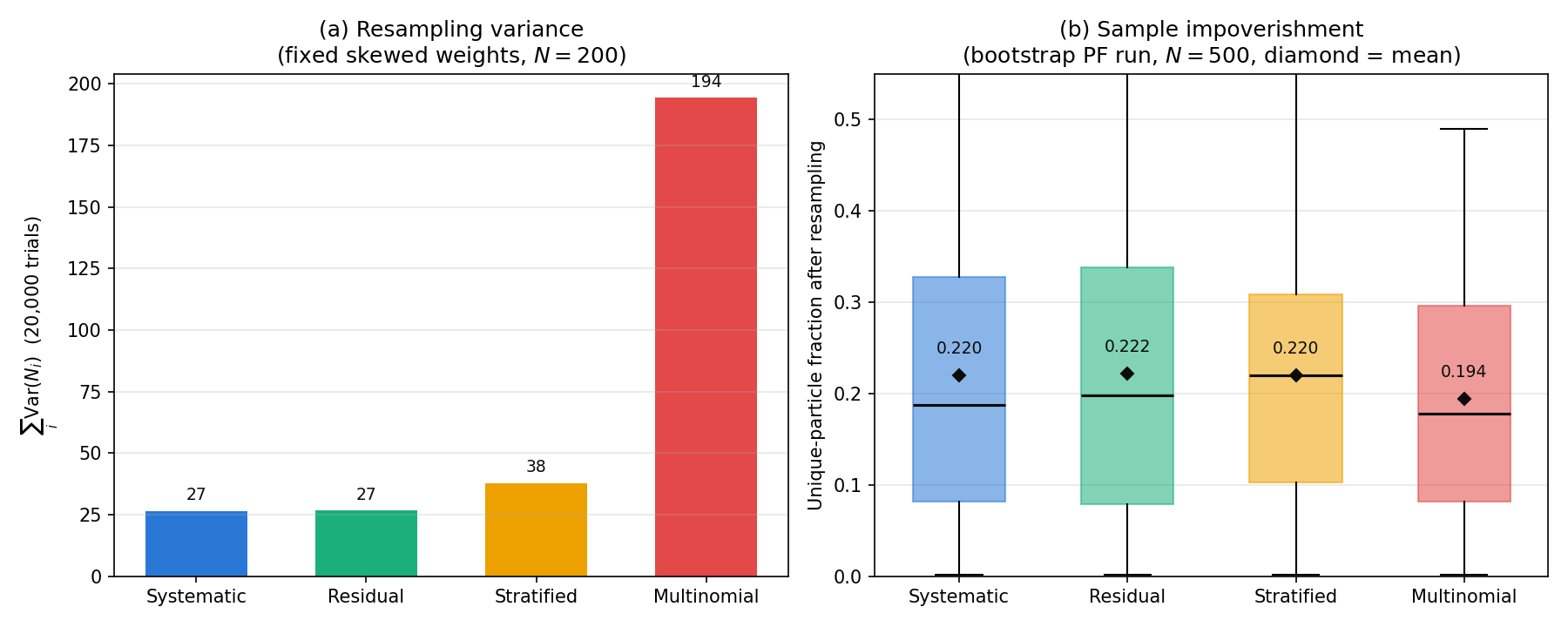
Every method loses roughly 78%–81% of its particle values per resampling event on average. The low-variance methods (systematic, residual, stratified) each retain about 22% unique particles, while multinomial resampling retains a somewhat lower 19.4% — confirming that the theoretical difference in offspring-count variance derived in the previous section also shows up as a real difference in particle diversity. That said, because this model’s process noise (\(\sigma_w = \sqrt{10}\) ) is large, diversity is quickly regenerated at the next step, so the degradation never becomes severe — which is part of why the RMSE comparison in the previous section showed only small differences between methods.
The Curse of Dimensionality: A Theoretical Lower Bound
The “difficult in high dimensions” property mentioned in the algorithm overview is not just intuition — it was proven as a theorem by Bengtsson, Bickel & Li (2008). They showed that as both the state dimension \(n\) and the particle count \(N\) grow (under mild assumptions, such as the observation likelihood having i.i.d. components), the maximum weight \(\max_i \tilde{w}^{(i)}\) converges to 1 — meaning nearly all probability mass concentrates on a single particle. Specifically, this collapse is unavoidable unless the particle count \(N\) grows exponentially in the dimension \(n\) (or, in a special case, exponentially in \(n^{1/3}\) ). In other words, doubling the dimension does not just require doubling the particle count — it requires an exponential increase in particle count relative to dimension.
This theoretical prediction is empirically confirmed in the Ensemble Kalman Filter article using a 40-dimensional Lorenz-96 model: increasing the particle count 50-fold, from \(N=20\) to \(N=1000\) , only improves the effective sample size from an average of 3.48 to 20.12 — barely changing as a fraction of \(N\) (EnKF, which does not use importance weights, is not subject to this constraint). This is precisely why the particle filter in this article suits low-dimensional, strongly nonlinear problems, while weighting-free methods like EnKF or UKF should be considered for high-dimensional problems.
Choosing the Resampling Threshold
This article uses \(N_{\text{eff}} < N/2\) as the resampling threshold, but this is a heuristic, not a universal rule. Setting the threshold lower (e.g., \(N/10\) ) reduces the frequency of resampling and mitigates sample impoverishment, but the filter then spends more steps with degenerate weights, increasing estimator variance. Setting the threshold higher (e.g., resampling at every step) minimizes degeneracy but accelerates sample impoverishment. This threshold choice and the choice of a low-variance resampling method (systematic, residual) are independent design decisions — both need to be made carefully for the particle filter to run stably.
Mismatch Between the Proposal and the Prior
This article’s implementation samples the initial particles from \(\mathcal{N}(0, 5)\) (standard deviation \(\approx 2.24\) ), while the true state fluctuates over a range of roughly \(\pm 20\) . If the prior does not adequately cover the range of the true state, all particles can simultaneously receive low likelihood at the initial step, causing severe degeneracy right at \(k=0\) . In practice, it is important to check the balance between the width of the prior and the size of the observation noise ahead of time.
Differentiable Resampling: Extending to Gradient-Based Learning
The systematic, stratified, and multinomial resampling methods in this article all involve a threshold comparison against the CDF (if positions[i] < cumsum[j]) or categorical sampling via np.random.choice — operations that are not differentiable with respect to the input weights. This means that if you want to learn the state transition function \(f\)
, the observation function \(h\)
, or the proposal distribution itself using a neural network, gradients are blocked at the resampling step. This has become an active research area in the 2020s. Most recently, Csuzdi, Törő & Bécsi (2024) proposed “Optimal Placement Resampling,” which reformulates deterministic sampling from the empirical CDF into a differentiable form, and applied it to gradient-based parameter estimation and proposal-distribution learning. It is notable that this method — conceptually close to the systematic resampling in this article (placing deterministic points on the CDF) — has been redesigned to be compatible with automatic differentiation, showing that classical resampling methods continue to be extended toward integration with deep learning.
Comparison of Filtering Methods
The following table compares the particle filter with Gaussian-approximation filters.
| Property | Particle Filter | UKF | CKF |
|---|---|---|---|
| Distribution assumption | None (arbitrary) | Gaussian | Gaussian |
| Computational cost | \(O(N)\) (depends on particle count) | \(O(n^3)\) | \(O(n^3)\) |
| Parameters | Particle count \(N\) , ESS threshold | \(\alpha, \beta, \kappa\) | None |
| Multimodality | Supported | Not supported | Not supported |
| High dimensions | Difficult (curse of dimensionality) | Good | Good |
| Implementation complexity | Moderate | Moderate | Low |
The particle filter’s key advantage is its freedom from distributional assumptions, but it faces the “curse of dimensionality” in high-dimensional problems where the required number of particles grows exponentially. For low-dimensional problems with strong nonlinearity or non-Gaussianity, the particle filter is the method of choice. For high-dimensional problems with moderate nonlinearity, CKF or UKF are more practical.
Related Articles
- Kalman Filter: Theory and Python Implementation - The optimal filter for linear Gaussian systems.
- Extended Kalman Filter (EKF): Theory and Python Implementation - Linearization-based approach for nonlinear systems.
- Unscented Kalman Filter (UKF): Nonlinear State Estimation Theory and Python Implementation - Sigma-point based nonlinear filter.
- Kalman Smoother (RTS Smoother): Theory and Python Implementation - Smoothing using observations from all time steps.
- Kalman Smoother Comparison - Cross-method comparison of Kalman smoothing approaches that leads into particle smoothing.
- Nonlinear Kalman Smoothers (Extended RTS Smoother, Unscented RTS Smoother) - Extends EKF/UKF to smoothing; a useful comparison point against particle smoothers when nonlinearity is strong but non-Gaussianity is moderate.
- Markov Chain Monte Carlo (MCMC): Metropolis-Hastings and Gibbs Sampling - A Monte Carlo sampling method closely related to particle filters.
- Monte Carlo Optimization Methods Comparison (CEM/SA/GA/MPPI/PSO) - Hub article applying the same importance-sampling framework used in particle filters to optimization across five methods, contrasting state estimation with function optimization.
- Machine Learning Hub for Time-Series, Classification, and Anomaly Detection - Hub article placing particle filters alongside linear Kalman, EKF, UKF, LSTM, and Isolation Forest, with guidance for non-Gaussian, strongly nonlinear state-space anomaly detection and forecasting.
- Ensemble Kalman Filter (EnKF): Theory and Python Implementation - Avoids this article’s curse of dimensionality using a weighting-free ensemble covariance approximation; directly compares both methods’ behavior on the 40-dimensional Lorenz-96 model.
References
- Arulampalam, M. S., Maskell, S., Gordon, N., & Clapp, T. (2002). “A Tutorial on Particle Filters for Online Nonlinear/Non-Gaussian Bayesian Tracking.” IEEE Transactions on Signal Processing, 50(2), 174-188.
- Doucet, A., & Johansen, A. M. (2009). “A Tutorial on Particle Filtering and Smoothing: Fifteen Years Later.” Handbook of Nonlinear Filtering, 12(656-704), 3.
- Douc, R., & Cappe, O. (2005). “Comparison of Resampling Schemes for Particle Filtering.” Proceedings of the 4th International Symposium on Image and Signal Processing and Analysis, 64-69.
- Gordon, N. J., Salmond, D. J., & Smith, A. F. M. (1993). “Novel Approach to Nonlinear/Non-Gaussian Bayesian State Estimation.” IEE Proceedings F (Radar and Signal Processing), 140(2), 107-113.
- Kong, A., Liu, J. S., & Wong, W. H. (1994). “Sequential Imputations and Bayesian Missing Data Problems.” Journal of the American Statistical Association, 89(425), 278-288.
- Doucet, A., Godsill, S., & Andrieu, C. (2000). “On Sequential Monte Carlo Sampling Methods for Bayesian Filtering.” Statistics and Computing, 10(3), 197-208.
- Bengtsson, T., Bickel, P., & Li, B. (2008). “Curse-of-Dimensionality Revisited: Collapse of the Particle Filter in Very Large Scale Systems.” IMS Collections: Probability and Statistics: Essays in Honor of David A. Freedman, 2, 316-334.
- Csuzdi, D., Törő, O., & Bécsi, T. (2024). “Differentiable Particle Filtering Using Optimal Placement Resampling.” arXiv preprint arXiv:2402.16639.