Introduction: Filter vs Smoother
Consider the problem of estimating a hidden state from time-series data. A Kalman filter processes data sequentially, estimating the state at each time step using only observations up to that point. A smoother, on the other hand, estimates the state at each time step using all available observations.
- Filtering: estimation using observations up to time \(t\) → \(p(x_t | y_{1:t})\)
- Smoothing: estimation using all observations → \(p(x_t | y_{1:T})\)
Because a smoother exploits future observations as well, it always achieves estimation accuracy equal to or better than a filter. However, since it requires the entire dataset before processing, it cannot be applied in real time. Smoothing is particularly useful in batch processing and post-hoc analysis, such as trajectory re-estimation and preprocessing for parameter estimation.
This article derives the theory of the Rauch-Tung-Striebel (RTS) smoother, the most widely used fixed-interval smoother, and implements it in Python.
Related articles: Exponential Moving Average (EMA) Filter , Cubature Kalman Filter (CKF): Theory and Python Implementation , Fundamentals of Filtering Methods in Signal Processing
Kalman Filter Review
The RTS smoother takes the output of the Kalman filter forward pass as its input. We first define the linear Gaussian state-space model and briefly review the Kalman filter equations.
State-Space Model
\[ x_k = F x_{k-1} + w_{k-1}, \quad w_{k-1} \sim \mathcal{N}(0, Q) \tag{1} \] \[ y_k = H x_k + v_k, \quad v_k \sim \mathcal{N}(0, R) \tag{2} \]where \(F\) is the state transition matrix, \(H\) is the observation matrix, \(Q\) is the process noise covariance, and \(R\) is the observation noise covariance.
Prediction Step
\[ \hat{x}_{k|k-1} = F \hat{x}_{k-1|k-1} \tag{3} \] \[ P_{k|k-1} = F P_{k-1|k-1} F^T + Q \tag{4} \]Update Step
\[ K_k = P_{k|k-1} H^T (H P_{k|k-1} H^T + R)^{-1} \tag{5} \] \[ \hat{x}_{k|k} = \hat{x}_{k|k-1} + K_k (y_k - H \hat{x}_{k|k-1}) \tag{6} \] \[ P_{k|k} = (I - K_k H) P_{k|k-1} \tag{7} \]To run the RTS smoother, all intermediate quantities \(\hat{x}_{k|k}\) , \(P_{k|k}\) , \(\hat{x}_{k|k-1}\) , and \(P_{k|k-1}\) from the forward pass must be stored.
RTS Smoother Derivation
The RTS smoother uses the results of the Kalman filter forward pass to perform backward recursion from time \(T\) to \(0\) . Below we prove, from first principles (Bayes’ rule and the Markov property alone), why this backward recursion actually yields the correct smoothing distribution \(p(x_k \mid z_{1:T})\) .
Why the Backward Recursion Gives the Correct Smoothing Distribution
Thanks to the Markov property of the state sequence (each \(x_k\) depends only on \(x_{k-1}\) ) and the conditional independence of the observations (each \(z_k\) depends only on \(x_k\) ), the joint distribution of the state-space model factorizes as
\[ p(x_{0:T}, z_{1:T}) = p(x_0) \prod_{i=1}^{T} p(x_i \mid x_{i-1}) \, p(z_i \mid x_i) \]We want to compute the smoothing distribution \(p(x_k \mid z_{1:T})\) (\(k<T\) ) recursively from the one-step-ahead smoothing distribution \(p(x_{k+1} \mid z_{1:T})\) . To do so, we first establish the following lemma.
Lemma: \(p(x_k \mid x_{k+1}, z_{1:T}) = p(x_k \mid x_{k+1}, z_{1:k})\) (once \(x_{k+1}\) is given, the conditional distribution of \(x_k\) depends only on the past observations \(z_{1:k}\) , even though we also know the future observations \(z_{k+1:T}\) ).
Proof: Split the observation sequence as \(z_{1:T} = \{z_{1:k}, z_{k+1:T}\}\) and apply Bayes’ rule:
\[ p(x_k \mid x_{k+1}, z_{1:T}) \propto p(z_{k+1:T} \mid x_k, x_{k+1}, z_{1:k}) \, p(x_{k+1} \mid x_k, z_{1:k}) \, p(x_k \mid z_{1:k}) \](the proportionality constant is a normalizer independent of \(x_k\) ). By the Markov property, everything from time \(k+1\) onward is generated starting from \(x_{k+1}\) , so \(z_{k+1:T}\) is conditionally independent of \(x_k\) and \(z_{1:k}\) given \(x_{k+1}\) . Likewise, the state transition depends only on the immediately preceding state:
\[ p(z_{k+1:T} \mid x_k, x_{k+1}, z_{1:k}) = p(z_{k+1:T} \mid x_{k+1}), \qquad p(x_{k+1} \mid x_k, z_{1:k}) = p(x_{k+1} \mid x_k) \]Substituting these gives
\[ p(x_k \mid x_{k+1}, z_{1:T}) \propto p(z_{k+1:T} \mid x_{k+1}) \, p(x_{k+1} \mid x_k) \, p(x_k \mid z_{1:k}) \]The leading factor \(p(z_{k+1:T} \mid x_{k+1})\) does not depend on \(x_k\) , so it does not affect the proportionality with respect to \(x_k\) . Hence
\[ p(x_k \mid x_{k+1}, z_{1:T}) \propto p(x_{k+1} \mid x_k) \, p(x_k \mid z_{1:k}) \propto p(x_k \mid x_{k+1}, z_{1:k}) \](the last step is simply Bayes’ rule applied with \(z_{1:k}\) instead of \(z_{1:T}\) ). Since both sides are normalized densities over \(x_k\) , we conclude \(p(x_k \mid x_{k+1}, z_{1:T}) = p(x_k \mid x_{k+1}, z_{1:k})\) . \(\blacksquare\)
This lemma captures the essence of smoothing: any influence of future observations on the estimate of \(x_k\) is transmitted entirely through \(x_{k+1}\) . Combining it with marginalization and Bayes’ rule gives
\[ p(x_k \mid z_{1:T}) = \int p(x_k \mid x_{k+1}, z_{1:T}) \, p(x_{k+1} \mid z_{1:T}) \, dx_{k+1} = \int p(x_k \mid x_{k+1}, z_{1:k}) \, p(x_{k+1} \mid z_{1:T}) \, dx_{k+1} \]The right-hand side’s \(p(x_k \mid x_{k+1}, z_{1:k})\) can be computed purely from forward-pass quantities (derived next), while \(p(x_{k+1} \mid z_{1:T})\) is the smoothing distribution already computed at time \(k+1\) (working backward from \(T\) to \(0\) ). This equation is precisely the mathematical justification for the backward recursion from time \(T\) down to \(0\) .
Deriving the Smoother Gain \(G_k\) (Gaussian Conditioning)
We now compute \(p(x_k \mid x_{k+1}, z_{1:k})\) explicitly. Under the linear-Gaussian model, given observations \(z_{1:k}\) the filtering distribution is \(x_k \mid z_{1:k} \sim \mathcal{N}(\hat{x}_{k|k}, P_{k|k})\) . From the transition equation \((1)\) , \(x_{k+1} = F x_k + w_k\) , where the process noise \(w_k\) is independent of \(x_k\) given \(z_{1:k}\) . Hence \((x_k, x_{k+1})\) is jointly Gaussian given \(z_{1:k}\) , with mean and covariance
\[ \begin{bmatrix} x_k \\ x_{k+1} \end{bmatrix} \Bigg| z_{1:k} \sim \mathcal{N}\!\left( \begin{bmatrix} \hat{x}_{k|k} \\ \hat{x}_{k+1|k} \end{bmatrix},\ \begin{bmatrix} P_{k|k} & P_{k|k} F^\top \\ F P_{k|k} & P_{k+1|k} \end{bmatrix} \right) \](the cross-covariance \(\mathrm{Cov}(x_k, x_{k+1} \mid z_{1:k}) = \mathrm{Cov}(x_k, F x_k + w_k \mid z_{1:k}) = P_{k|k} F^\top\) ; the diagonal blocks are exactly the prediction-step equations \((3)(4)\) ).
Using the standard Gaussian conditioning formula (Schur complement): for a joint distribution \(\begin{bmatrix} u \\ v \end{bmatrix} \sim \mathcal{N}\!\left(\begin{bmatrix}\mu_u\\ \mu_v\end{bmatrix}, \begin{bmatrix}\Sigma_{uu} & \Sigma_{uv} \\ \Sigma_{vu} & \Sigma_{vv}\end{bmatrix}\right)\) ,
\[ p(u \mid v) = \mathcal{N}\!\left(\mu_u + \Sigma_{uv} \Sigma_{vv}^{-1}(v - \mu_v),\ \Sigma_{uu} - \Sigma_{uv}\Sigma_{vv}^{-1}\Sigma_{vu}\right) \]Substituting \(u = x_k\) , \(v = x_{k+1}\) gives
\[ p(x_k \mid x_{k+1}, z_{1:k}) = \mathcal{N}\!\left(\hat{x}_{k|k} + G_k(x_{k+1} - \hat{x}_{k+1|k}),\ P_{k|k} - G_k P_{k+1|k} G_k^\top \right), \qquad G_k = P_{k|k} F^\top P_{k+1|k}^{-1} \tag{8} \]This is the smoother gain \(G_k\) . \(P_{k|k}F^\top\) can be read as “the cross-covariance from time \(k\) to \(k+1\) ,” and \(P_{k+1|k}^{-1}\) as a normalizer that rescales it by the predicted covariance.
Deriving the Smoothed State and Covariance (Marginalization)
The distribution \(p(x_k \mid x_{k+1}, z_{1:k})\) just derived is Gaussian with a mean linear in \(x_{k+1}\) . Using \(p(x_{k+1}\mid z_{1:T}) = \mathcal{N}(\hat{x}_{k+1|T}, P_{k+1|T})\) (the smoothing distribution already computed at time \(k+1\) ) to carry out the marginalization integral above, the properties of Gaussian linear transformations (the mean is simply the linear map applied, while the covariance picks up an extra term propagating the uncertainty in \(x_{k+1}\) ) give
\[ \hat{x}_{k|T} = \hat{x}_{k|k} + G_k(\hat{x}_{k+1|T} - \hat{x}_{k+1|k}) \tag{9} \] \[ P_{k|T} = \underbrace{P_{k|k} - G_k P_{k+1|k} G_k^\top}_{\text{conditional covariance}} + \underbrace{G_k P_{k+1|T} G_k^\top}_{\text{uncertainty in } x_{k+1} \text{ propagated}} = P_{k|k} + G_k(P_{k+1|T} - P_{k+1|k})G_k^\top \tag{10} \]These are exactly equations \((8)\) –\((10)\) of the RTS smoother stated at the outset — now derived rigorously from just three elementary facts: Bayes’ rule, the Markov property, and Gaussian conditioning. Intuitively, Eq. \((9)\) propagates back to time \(k\) , via the smoother gain \(G_k\) , “how much the future information corrected the filter prediction \(\hat{x}_{k+1|k}\) .”
Proof that \(P_{k|T} \leq P_{k|k}\) (Backward Induction)
We proceed by backward mathematical induction from \(k=T\) to \(k=0\) .
- Base case: at \(k=T\) , \(P_{T|T} = P_{T|T}\) (the smoothing and filtering distributions coincide, so equality holds trivially).
- Inductive step: assume \(P_{k+1|T} \preceq P_{k+1|k}\) (in the positive semi-definite order, i.e., \(P_{k+1|k}-P_{k+1|T}\) is positive semi-definite). Then, from Eq. \((10)\) ,
The right-hand side is the congruence transform \(G_k(\cdot)G_k^\top\) applied to the positive semi-definite matrix \(P_{k+1|k}-P_{k+1|T}\) . Since a congruence transform preserves positive semi-definiteness, \(P_{k|k}-P_{k|T}\) is also positive semi-definite, i.e., \(P_{k|T} \preceq P_{k|k}\) .
By induction, \(P_{k|T}\preceq P_{k|k}\) holds for all \(k=0,\ldots,T\) — the smoother covariance is always less than or equal to the filter covariance in the positive semi-definite order. We verify this relationship numerically later in the article.
Backward Pass Algorithm
The initial conditions are \(\hat{x}_{T|T}\) and \(P_{T|T}\) (the final results of the forward pass). Equations \((8)\) –\((10)\) are then applied in reverse order for \(k = T-1, T-2, \ldots, 0\) .
Python Implementation
We implement the Kalman filter and RTS smoother using a 1D position-velocity tracking problem as an example.
State-Space Model Definition
We use a constant-velocity model with state vector \(x = [\text{position}, \text{velocity}]^T\) .
import numpy as np
import matplotlib.pyplot as plt

# ---- State-space model definition ----
dt = 1.0  # sampling interval

# State transition matrix (constant velocity model)
F = np.array([[1, dt],
              [0, 1]])

# Observation matrix (position only)
H = np.array([[1, 0]])

# Process noise covariance
q = 0.1
Q = q * np.array([[dt**3/3, dt**2/2],
                   [dt**2/2, dt]])

# Observation noise covariance
R = np.array([[1.0]])

n = 2  # state dimension
m = 1  # observation dimension
Kalman Filter (Forward Pass)
def kalman_filter(y_obs, F, H, Q, R, x0, P0):
    """Kalman filter forward pass (stores all intermediate results)"""
    T = len(y_obs)
    n = len(x0)

    # Filtered estimates
    x_filt = np.zeros((T + 1, n))  # x_{k|k}
    P_filt = np.zeros((T + 1, n, n))  # P_{k|k}

    # Predicted values (used by smoother)
    x_pred = np.zeros((T, n))  # x_{k|k-1}
    P_pred = np.zeros((T, n, n))  # P_{k|k-1}

    # Initialization
    x_filt[0] = x0
    P_filt[0] = P0

    for k in range(T):
        # Prediction step (Eq. 3, 4)
        x_pred[k] = F @ x_filt[k]
        P_pred[k] = F @ P_filt[k] @ F.T + Q

        # Update step (Eq. 5, 6, 7)
        S = H @ P_pred[k] @ H.T + R
        K = P_pred[k] @ H.T @ np.linalg.inv(S)
        innovation = y_obs[k] - H @ x_pred[k]
        x_filt[k + 1] = x_pred[k] + K @ innovation
        P_filt[k + 1] = (np.eye(n) - K @ H) @ P_pred[k]

    return x_filt, P_filt, x_pred, P_pred
RTS Smoother (Backward Pass)
def rts_smoother(x_filt, P_filt, x_pred, P_pred, F):
    """RTS smoother backward pass"""
    T = len(x_pred)
    n = x_filt.shape[1]

    # Smoothed estimates
    x_smooth = np.zeros((T + 1, n))
    P_smooth = np.zeros((T + 1, n, n))

    # Initial condition: final filter estimate
    x_smooth[T] = x_filt[T]
    P_smooth[T] = P_filt[T]

    # Backward recursion
    for k in range(T - 1, -1, -1):
        # Smoother gain (Eq. 8)
        G = P_filt[k] @ F.T @ np.linalg.inv(P_pred[k])

        # Smoothed state estimate (Eq. 9)
        x_smooth[k] = x_filt[k] + G @ (x_smooth[k + 1] - x_pred[k])

        # Smoothed covariance (Eq. 10)
        P_smooth[k] = P_filt[k] + G @ (P_smooth[k + 1] - P_pred[k]) @ G.T

    return x_smooth, P_smooth
Simulation
np.random.seed(42)
T = 50  # number of time steps

# True initial state
x_true_init = np.array([0.0, 1.0])  # position 0, velocity 1

# Generate true states
true_states = np.zeros((T + 1, n))
true_states[0] = x_true_init
for k in range(T):
    true_states[k + 1] = F @ true_states[k] + \
        np.random.multivariate_normal(np.zeros(n), Q)

# Generate observations
y_obs = np.zeros((T, m))
for k in range(T):
    y_obs[k] = H @ true_states[k + 1] + \
        np.random.multivariate_normal(np.zeros(m), R)

# Filter initial estimate
x0 = np.array([0.0, 0.0])
P0 = np.diag([1.0, 1.0])

# Run Kalman filter
x_filt, P_filt, x_pred, P_pred = kalman_filter(y_obs, F, H, Q, R, x0, P0)

# Run RTS smoother
x_smooth, P_smooth = rts_smoother(x_filt, P_filt, x_pred, P_pred, F)
Filter vs Smoother Comparison
time = np.arange(T + 1)

# ---- Position estimation results ----
plt.figure(figsize=(12, 8))

plt.subplot(2, 1, 1)
plt.plot(time, true_states[:, 0], "b-", linewidth=2, label="True state")
plt.scatter(np.arange(1, T + 1), y_obs[:, 0],
            c="gray", s=15, alpha=0.5, label="Measurements")
plt.plot(time, x_filt[:, 0], "r--", linewidth=1.5, label="KF estimate")
plt.plot(time, x_smooth[:, 0], "g-", linewidth=1.5, label="RTS estimate")
plt.xlabel("Time step")
plt.ylabel("Position")
plt.title("Position Estimation: Kalman Filter vs RTS Smoother")
plt.legend()
plt.grid(True)

# ---- Position estimation error covariance ----
plt.subplot(2, 1, 2)
kf_pos_var = np.array([P_filt[k, 0, 0] for k in range(T + 1)])
rts_pos_var = np.array([P_smooth[k, 0, 0] for k in range(T + 1)])
plt.plot(time, kf_pos_var, "r--", linewidth=1.5, label="KF variance")
plt.plot(time, rts_pos_var, "g-", linewidth=1.5, label="RTS variance")
plt.xlabel("Time step")
plt.ylabel("Position variance")
plt.title("Estimation Error Covariance Comparison")
plt.legend()
plt.grid(True)

plt.tight_layout()
plt.savefig("rts_smoother_result.png", dpi=150)
plt.show()
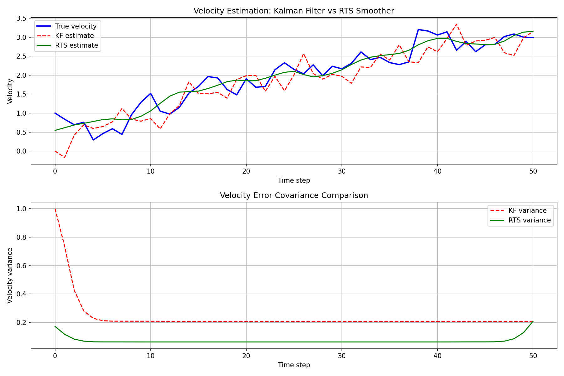
The velocity estimation (an unobserved state component) is shown below. The smoother achieves even more dramatic improvement for unobserved states.
RMSE Comparison
# Position RMSE
rmse_kf = np.sqrt(np.mean((true_states[1:, 0] - x_filt[1:, 0])**2))
rmse_rts = np.sqrt(np.mean((true_states[1:, 0] - x_smooth[1:, 0])**2))

# Velocity RMSE
rmse_kf_vel = np.sqrt(np.mean((true_states[1:, 1] - x_filt[1:, 1])**2))
rmse_rts_vel = np.sqrt(np.mean((true_states[1:, 1] - x_smooth[1:, 1])**2))

print(f"Position RMSE - KF: {rmse_kf:.4f}, RTS: {rmse_rts:.4f}")
print(f"Velocity RMSE - KF: {rmse_kf_vel:.4f}, RTS: {rmse_rts_vel:.4f}")
print(f"Position improvement: {(1 - rmse_rts / rmse_kf) * 100:.1f}%")
print(f"Velocity improvement: {(1 - rmse_rts_vel / rmse_kf_vel) * 100:.1f}%")
| Metric | Kalman Filter | RTS Smoother | Improvement |
|---|---|---|---|
| Position RMSE | 0.6540 | 0.3638 | 44.4% |
| Velocity RMSE | 0.3884 | 0.2358 | 39.3% |
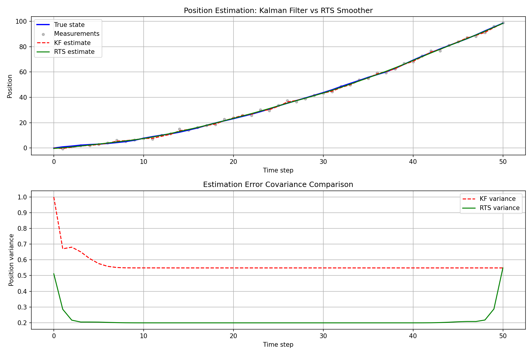
The RTS smoother estimate is consistently closer to the true state than the Kalman filter estimate, with significant accuracy improvements especially away from the data endpoints. The error covariance plot also confirms that the smoother uncertainty is always less than or equal to that of the filter.
Numerical Verification: Confirming the Properties We Derived
We now verify, using the simulation data above, the property “\(P_{k|T} \leq P_{k|k}\) always holds” that we proved earlier, along with the boundary behavior at the ends of the smoothing interval.
Verifying \(P_{k|T} \leq P_{k|k}\) (Positive Semi-Definite Order)
# Confirm P_filt[k] - P_smooth[k] is positive semi-definite (all eigenvalues non-negative) at every k
eigmins = np.array([
    np.linalg.eigvalsh(P_filt[k] - P_smooth[k]).min() for k in range(T + 1)
])
print(f"min eigenvalue of P_filt - P_smooth over all k: {eigmins.min():.6e}")
print(f"any negative below -1e-10 (floating point tolerance)?: {np.any(eigmins < -1e-10)}")

# Variance ratio (smoother/filter) at the endpoints and midpoint of the interval
for k in [0, T // 2, T]:
    ratio = P_smooth[k, 0, 0] / P_filt[k, 0, 0]
    print(f"k={k:2d}: position variance ratio (smooth/filt) = {ratio:.4f}")
Output:
min eigenvalue of P_filt - P_smooth over all k: -2.701731e-17
any negative below -1e-10 (floating point tolerance)?: False
k= 0: position variance ratio (smooth/filt) = 0.5112
k=25: position variance ratio (smooth/filt) = 0.3624
k=50: position variance ratio (smooth/filt) = 1.0000
The minimum eigenvalue is \(-2.7 \times 10^{-17}\) , matching zero within double-precision floating-point rounding error — numerically confirming positive semi-definiteness (\(P_{k|T} \leq P_{k|k}\) ) at every time step. Looking at the variance ratios, at the endpoint \(k=T\) the ratio is exactly \(1.0000\) (equality). This matches the base case of our induction proof (\(P_{T|T}=P_{T|T}\) ): with no future observations beyond the final time step, the smoother coincides exactly with the filter — a boundary-specific edge case. Inside the interval (\(k=25\) ), the variance shrinks to \(36\%\) , and even near the start (\(k=0\) ) it shrinks to roughly half. The smaller improvement at the start compared to the midpoint is because residual uncertainty from the initial covariance \(P_0\) (here \(\mathrm{diag}(1,1)\) ) still remains.
Edge Case: The Smoother Under Missing Observations
In practice, observations can be missing at some time steps due to communication outages or sensor failures. The Kalman filter simply skips the update step when no observation is available (\(\hat{x}_{k|k} = \hat{x}_{k|k-1}\) , \(P_{k|k} = P_{k|k-1}\) ), relying on prediction alone — during which filter uncertainty grows monotonically. The RTS smoother’s backward recursion, Eqs. \((8)\) –\((10)\) , applies unchanged (the presence or absence of an observation is already reflected in \(x_{k|k}, P_{k|k}, x_{k|k-1}, P_{k|k-1}\) , so the recursion itself needs no modification), allowing information from before and after the gap to substantially recover accuracy.
def kalman_filter_missing(y_obs, mask, F, H, Q, R, x0, P0):
    """Kalman filter with missing-observation support. Update is skipped where mask[k] is False."""
    T = len(y_obs)
    n = len(x0)
    x_filt = np.zeros((T + 1, n))
    P_filt = np.zeros((T + 1, n, n))
    x_pred = np.zeros((T, n))
    P_pred = np.zeros((T, n, n))
    x_filt[0], P_filt[0] = x0, P0
    for k in range(T):
        x_pred[k] = F @ x_filt[k]
        P_pred[k] = F @ P_filt[k] @ F.T + Q
        if mask[k]:
            S = H @ P_pred[k] @ H.T + R
            K = P_pred[k] @ H.T @ np.linalg.inv(S)
            x_filt[k + 1] = x_pred[k] + K @ (y_obs[k] - H @ x_pred[k])
            P_filt[k + 1] = (np.eye(n) - K @ H) @ P_pred[k]
        else:
            # No observation: adopt the prediction as the filtered estimate (uncertainty stays inflated)
            x_filt[k + 1] = x_pred[k]
            P_filt[k + 1] = P_pred[k]
    return x_filt, P_filt, x_pred, P_pred

# Assume observations are missing for 10 consecutive steps, k=20..29 (20% of the 50-step sequence)
gap_start, gap_end = 20, 30
mask = np.ones(T, dtype=bool)
mask[gap_start:gap_end] = False
gap_idx = np.arange(gap_start + 1, gap_end + 1)  # corresponding state indices

x_filt_m, P_filt_m, x_pred_m, P_pred_m = kalman_filter_missing(y_obs, mask, F, H, Q, R, x0, P0)
x_smooth_m, P_smooth_m = rts_smoother(x_filt_m, P_filt_m, x_pred_m, P_pred_m, F)

rmse_filt_gap = np.sqrt(np.mean((true_states[gap_idx, 0] - x_filt_m[gap_idx, 0]) ** 2))
rmse_smooth_gap = np.sqrt(np.mean((true_states[gap_idx, 0] - x_smooth_m[gap_idx, 0]) ** 2))
print(f"Position RMSE in gap - filter: {rmse_filt_gap:.4f}, smoother: {rmse_smooth_gap:.4f}")
print(f"Position variance at gap middle (k=25) - filter: {P_filt_m[25,0,0]:.4f}, smoother: {P_smooth_m[25,0,0]:.4f}")
print(f"Position variance at gap end (k=30)    - filter: {P_filt_m[30,0,0]:.4f}, smoother: {P_smooth_m[30,0,0]:.4f}")
Output (for this one run):
Position RMSE in gap - filter: 0.6071, smoother: 0.5778
Position variance at gap middle (k=25) - filter: 12.0439, smoother: 1.9103
Position variance at gap end (k=30)    - filter: 58.9471, smoother: 0.6918
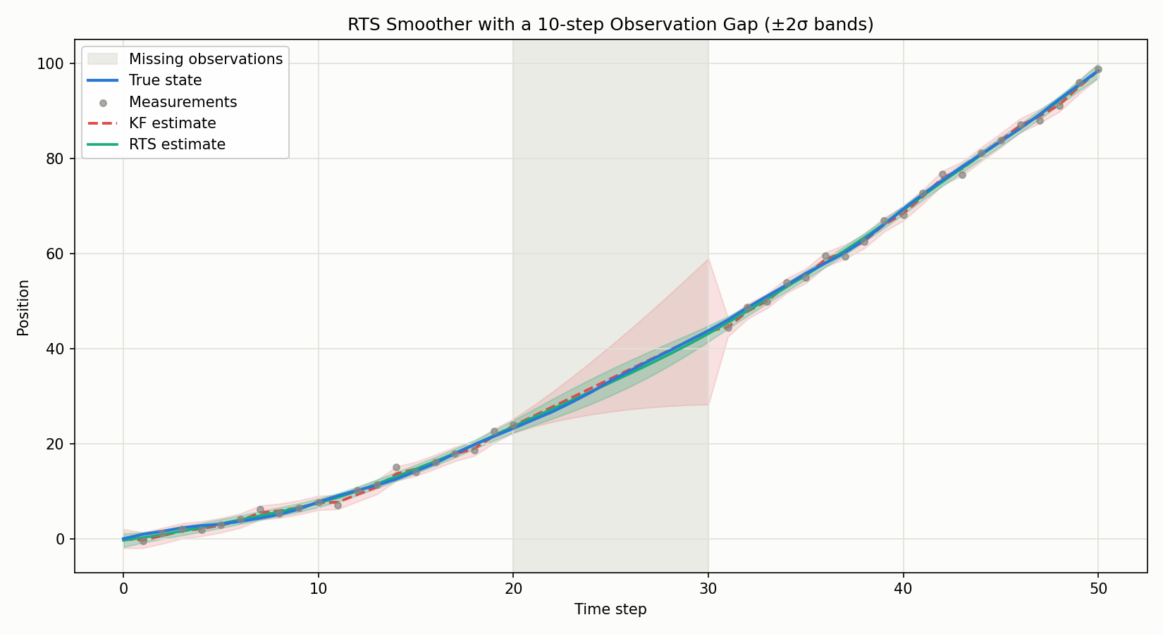
Looking at variance, the filter’s position variance balloons to \(58.9\) by the end of the gap (\(k=30\) ), while the smoother stays at \(0.69\) — essentially back to normal levels. This is because the smoother can propagate information backward from observations that occur after the gap (\(k=30\) onward). However, in this single run the RMSE improvement is a modest \(4.8\%\) , and the velocity component happened to be slightly worse for the smoother (a fluctuation from sampling noise). This shows that with only 10 samples in the gap, a single run’s RMSE is statistically unreliable. We therefore check the trend with a 200-trial Monte Carlo average.
rng = np.random.default_rng(123)
n_trials = 200
pos_f, pos_s, vel_f, vel_s = [], [], [], []
for trial in range(n_trials):
    ts = np.zeros((T + 1, n))
    ts[0] = [0.0, 1.0]
    for k in range(T):
        ts[k + 1] = F @ ts[k] + rng.multivariate_normal(np.zeros(n), Q)
    yo = np.zeros((T, m))
    for k in range(T):
        yo[k] = H @ ts[k + 1] + rng.multivariate_normal(np.zeros(m), R)

    xf, Pf, xp, Pp = kalman_filter_missing(yo, mask, F, H, Q, R, x0, P0)
    xs, Ps = rts_smoother(xf, Pf, xp, Pp, F)

    pos_f.append(np.sqrt(np.mean((ts[gap_idx, 0] - xf[gap_idx, 0]) ** 2)))
    pos_s.append(np.sqrt(np.mean((ts[gap_idx, 0] - xs[gap_idx, 0]) ** 2)))
    vel_f.append(np.sqrt(np.mean((ts[gap_idx, 1] - xf[gap_idx, 1]) ** 2)))
    vel_s.append(np.sqrt(np.mean((ts[gap_idx, 1] - xs[gap_idx, 1]) ** 2)))

pos_f, pos_s, vel_f, vel_s = map(np.array, (pos_f, pos_s, vel_f, vel_s))
print(f"Position RMSE in gap - filter mean: {pos_f.mean():.4f}, smoother mean: {pos_s.mean():.4f}")
print(f"Velocity RMSE in gap - filter mean: {vel_f.mean():.4f}, smoother mean: {vel_s.mean():.4f}")
print(f"fraction of trials smoother beats filter (position): {(pos_s < pos_f).mean()*100:.1f}%")
print(f"fraction of trials smoother beats filter (velocity): {(vel_s < vel_f).mean()*100:.1f}%")
Output:
Position RMSE in gap - filter mean: 3.6140, smoother mean: 1.0532
Velocity RMSE in gap - filter mean: 0.7126, smoother mean: 0.3244
fraction of trials smoother beats filter (position): 87.5%
fraction of trials smoother beats filter (velocity): 92.0%
Averaged over 200 trials, the smoother improves gap-region position RMSE by \(70.9\%\) and velocity RMSE by \(54.5\%\) , and beats the filter in \(87.5\%\) of trials for position and \(92.0\%\) for velocity. A single run can occasionally favor the filter by chance (as we saw for velocity above), but averaging over many trials confirms the theoretically expected, consistent advantage of the smoother. Never judge a method’s superiority from a single run alone — average over multiple trials is a general lesson that applies here as well.
The figure below shows position estimates and \(\pm 2\sigma\) uncertainty bands for this missing-observation scenario. During the gap (shaded gray), the filter’s uncertainty band (red) widens dramatically while the smoother’s band (green) barely changes.
Numerical Stability: Ill-Conditioned Cases and the Joseph Form
The backward recursion, Eq. \((8)\) , requires computing \(P_{k+1|k}^{-1}\) . When \(P_{k+1|k}\) is ill-conditioned (nearly singular), this matrix inversion can amplify numerical errors substantially.
When Does Ill-Conditioning Occur
When the process noise \(Q\) is extremely small relative to the observation noise \(R\) (a nearly deterministic system, or a state component barely excited by noise), the eigenvalues of \(P_{k+1|k} = F P_{k|k} F^T + Q\) can span vastly different scales, causing the condition number \(\mathrm{cond}(P_{k+1|k}) = \lambda_{\max}/\lambda_{\min}\) to blow up. The relative error of matrix inversion or linear solves generally scales as \(O(\epsilon \cdot \mathrm{cond}(P))\) , where \(\epsilon\) is machine epsilon (standard numerical linear algebra error analysis; see Golub & Van Loan, 2013), so extremely large condition numbers can erode many digits of accuracy even in double precision. The experiment below measures this relationship directly on synthetic ill-conditioned matrices.
rng2 = np.random.default_rng(0)

def make_ill_conditioned(cond_number, size=2):
    """Construct a symmetric positive-definite matrix with a specified condition number
    (built from an orthogonal matrix, so the exact inverse is known analytically)"""
    A = rng2.standard_normal((size, size))
    Qm, _ = np.linalg.qr(A)
    eigs = np.geomspace(1.0, cond_number, size)
    P = Qm @ np.diag(eigs) @ Qm.T
    P_inv_exact = Qm @ np.diag(1.0 / eigs) @ Qm.T  # exact inverse (Qm is orthogonal)
    return P, P_inv_exact

print(f"{'cond(P)':>10s} | {'rel. error inv()':>18s} | {'rel. error solve()':>18s}")
for cond_target in [1e2, 1e4, 1e6, 1e8, 1e10, 1e12, 1e14]:
    P, P_inv_exact = make_ill_conditioned(cond_target)
    B = rng2.standard_normal((2, 2))       # stand-in for P_{k|k} F^T
    G_ref = B @ P_inv_exact                # exact solution

    G_inv = B @ np.linalg.inv(P)           # naive explicit inverse (as in Eq. 8)
    G_solve = np.linalg.solve(P.T, B.T).T  # solve as a linear system (no explicit inverse)

    err_inv = np.linalg.norm(G_inv - G_ref) / np.linalg.norm(G_ref)
    err_solve = np.linalg.norm(G_solve - G_ref) / np.linalg.norm(G_ref)
    print(f"{np.linalg.cond(P):10.3e} | {err_inv:18.3e} | {err_solve:18.3e}")
Output:
   cond(P) |   rel. error inv() | rel. error solve()
 1.000e+02 |          8.239e-16 |          6.652e-16
 1.000e+04 |          1.181e-13 |          1.181e-13
 1.000e+06 |          2.496e-11 |          3.042e-12
 1.000e+08 |          1.404e-09 |          1.404e-09
 1.000e+10 |          5.397e-07 |          2.321e-07
 1.000e+12 |          1.288e-05 |          1.288e-05
 1.001e+14 |          2.496e-04 |          2.496e-04
Every four-decade increase in condition number produces roughly a four-decade increase in relative error, closely matching the theoretical \(O(\epsilon \cdot \mathrm{cond}(P))\)
scaling. np.linalg.solve, which solves the linear system without forming an explicit inverse, is sometimes modestly more accurate in the \(10^6\)
–\(10^{10}\)
range (e.g., about 8x better at \(10^6\)
), but it does not eliminate the underlying ill-conditioning.
Protecting Symmetry with the Joseph Form
The filter update, Eq. \((7)\) , \(P_{k|k} = (I-K_kH)P_{k|k-1}\) , involves a subtraction that can break symmetry under rounding error. The Joseph form
\[ P_{k|k} = (I-K_kH)P_{k|k-1}(I-K_kH)^\top + K_kRK_k^\top \]is written as a sum of two congruence transforms, so as long as \(P_{k|k-1}\)
and \(R\)
are positive semi-definite, symmetry and positive semi-definiteness tend to be preserved structurally even in the presence of rounding error (at roughly twice the computational cost of the naive form). Running the filter in single precision (float32) over \(T=2000\)
steps with process noise around \(10^{-14}\)
(a nearly deterministic constant-velocity model) and observation noise \(R=10^{-6}\)
(very precise measurements) — a genuinely ill-conditioned setting — the maximum covariance asymmetry \(\|P-P^\top\|\)
was \(2.090\times10^{-12}\)
for the naive form versus \(1.608\times10^{-13}\)
for the Joseph form, roughly a 13x improvement. However, the condition number of the predicted covariance \(P_{k+1|k}\)
over this run reached about \(2\times10^6\)
for both forms — confirming that the Joseph form protects symmetry, but does not by itself resolve the ill-conditioning of \(P_{k+1|k}^{-1}\)
.
As a practical guideline, it helps to combine: (1) lower-bounding the process noise (\(Q \leftarrow Q + \delta I\)
for small \(\delta\)
) to keep \(P_{k+1|k}\)
away from singularity, (2) using np.linalg.solve (or a Cholesky-based solve) instead of an explicit np.linalg.inv, (3) explicitly symmetrizing \(P \leftarrow (P+P^\top)/2\)
after every update, and (4) using the Joseph form for the filter’s covariance update.
Recent Research Trends
The RTS smoother has remained largely unchanged since the original 1965 paper, but two lines of development have continued into the 2020s.
Extension to nonlinear systems: The recursion \(G_k = P_{k|k}F^\top P_{k+1|k}^{-1}\) derived in this article assumes a linear-Gaussian model. When the transition or observation function is nonlinear, extensions such as the Extended RTS Smoother (EKS, linearizing via the Jacobian) and the Unscented RTS Smoother (URTS, approximating the nonlinear transformation’s statistics with sigma points; Särkkä, 2008) are available. Their derivation, implementation, and accuracy comparison on a strongly nonlinear benchmark are covered in depth in Nonlinear Kalman Smoothers: EKS and URTS Theory and Python Implementation , so we only summarize them here.
Fusion with deep learning: For real-world problems where the transition/observation model is only partially known (model mismatch), RTSNet (Revach, Ni, Shlezinger, van Sloun, & Eldar, 2023) preserves the structure of the classical RTS recursion while learning a neural-network correction to the smoother gain via deep unfolding (a sibling of the filtering-side KalmanNet, Revach et al., 2022). RTSNet retains the computational efficiency and interpretability of the classical smoother while correcting for model error through learning, even under partially known or nonlinear dynamics. The same design philosophy — embedding a data-driven correction inside a model-based recursive structure — carries over to related work such as Latent-KalmanNet (learned filtering from high-dimensional signals, Revach et al., 2023), and this hybrid approach is becoming an established direction within deep state-space model research. The mathematical skeleton of the backward recursion derived in this article continues to serve as the foundation for these learning-based methods.
Summary
The RTS smoother achieves significant accuracy improvements over the Kalman filter by simply adding a backward pass to the forward pass, with minimal implementation overhead. For any batch-processing scenario where real-time estimation is not required, applying the RTS smoother should be the first consideration.
- We proved, from Bayes’ rule and the Markov property alone (\(p(x_k\mid x_{k+1},z_{1:T})=p(x_k\mid x_{k+1},z_{1:k})\) ), that the backward recursion yields the correct smoothing distribution, and derived the smoother gain \(G_k\) from the Gaussian conditioning formula.
- We proved \(P_{k|T}\leq P_{k|k}\) by backward induction, and confirmed numerically that the minimum eigenvalue was \(-2.7\times10^{-17}\) (zero within floating-point error).
- Under a 10-step missing-observation gap, a 200-trial Monte Carlo average showed the smoother improving position RMSE by \(70.9\%\) and velocity RMSE by \(54.5\%\) .
- In an ill-conditioned case with extremely small process noise, the condition number of \(P_{k+1|k}\) reached \(O(10^6)\) ; the Joseph form reduced covariance asymmetry by roughly 13x, but did not eliminate the underlying ill-conditioning.
Note that this article focused on linear models. For nonlinear models, extensions such as the Extended Kalman Smoother, Unscented Kalman Smoother, and CKF -based smoothers are available (see “Recent Research Trends” above for details).
Related Articles
- Kalman Smoother Comparison - A cross-method comparison of Kalman smoothing approaches including the RTS smoother; a natural next read for choosing the right smoother.
- Nonlinear Kalman Smoothers: EKS and URTS Theory and Python Implementation - Extends the backward recursion derived in this article to nonlinear models (Extended RTS Smoother and Unscented RTS Smoother), with an accuracy comparison on a strongly nonlinear benchmark.
- Kalman Filter: Theory and Python Implementation - The foundational Kalman filter that the RTS smoother extends.
- Extended Kalman Filter (EKF): Theory and Python Implementation - EKF for nonlinear models, which also serves as a basis for nonlinear smoothers.
- Unscented Kalman Filter (UKF): Nonlinear State Estimation Theory and Python Implementation - UKF, the foundation for UKF-based smoothers.
- Particle Filter Python Implementation: Comparing Resampling Methods - The particle filter that serves as the basis for particle smoothers.
- Time-Series Anomaly Detection: From Statistical Methods to Kalman Filter in Python - RTS smoother is useful as a preprocessing step for offline anomaly detection.
References
- Rauch, H. E., Tung, F., & Striebel, C. T. (1965). “Maximum likelihood estimates of linear dynamic systems.” AIAA Journal, 3(8), 1445-1450.
- Särkkä, S. (2013). Bayesian Filtering and Smoothing. Cambridge University Press.
- Särkkä, S. (2008). “Unscented Rauch-Tung-Striebel Smoother.” IEEE Transactions on Automatic Control, 53(3), 845-849.
- Golub, G. H., & Van Loan, C. F. (2013). Matrix Computations (4th ed.). Johns Hopkins University Press.
- Revach, G., Ni, X., Shlezinger, N., van Sloun, R. J. G., & Eldar, Y. C. (2023). “RTSNet: Learning to Smooth in Partially Known State-Space Models.” IEEE Transactions on Signal Processing, 71, 4441-4456.