What is the Extended Kalman Filter?
The Kalman Filter (KF) is the optimal state estimator for linear Gaussian systems, but most real-world systems are nonlinear. The Extended Kalman Filter (EKF) extends the KF framework to nonlinear systems by linearizing the nonlinear functions around the current estimate using Jacobian matrices (first-order Taylor expansion).
EKF is the most fundamental nonlinear filtering technique and serves as the starting point for more advanced methods:
- EKF: First-order linearization via Jacobian matrices
- UKF: Direct approximation of nonlinear transforms using sigma points (Unscented Transformation)
- CKF : Sigma point selection based on the spherical-radial cubature rule
- Particle Filter : Monte Carlo sampling to approximate arbitrary distributions
Nonlinear State-Space Model
Consider the following nonlinear state-space model:
\[ \mathbf{x}_k = f(\mathbf{x}_{k-1}) + \mathbf{w}_{k-1}, \quad \mathbf{w}_{k-1} \sim \mathcal{N}(\mathbf{0}, \mathbf{Q}) \tag{1} \] \[ \mathbf{z}_k = h(\mathbf{x}_k) + \mathbf{v}_k, \quad \mathbf{v}_k \sim \mathcal{N}(\mathbf{0}, \mathbf{R}) \tag{2} \]Here \(f\) is the nonlinear state transition function and \(h\) is the nonlinear observation function. In the linear KF, these are expressed as matrices (\(f(\mathbf{x}) = \mathbf{A}\mathbf{x}\) and \(h(\mathbf{x}) = \mathbf{H}\mathbf{x}\) ), but in the EKF they are general nonlinear functions.
Linearization via Jacobian Matrices
The key idea of the EKF is to perform a Taylor expansion of the nonlinear functions \(f\) and \(h\) around the current estimate, retaining only the first-order terms.
The Jacobian of the state transition function \(f\) is computed at the previous estimate \(\hat{\mathbf{x}}_{k-1|k-1}\) :
\[ \mathbf{F}_k = \frac{\partial f}{\partial \mathbf{x}}\bigg|_{\mathbf{x}=\hat{\mathbf{x}}_{k-1|k-1}} = \begin{bmatrix} \frac{\partial f_1}{\partial x_1} & \cdots & \frac{\partial f_1}{\partial x_n} \\\ \vdots & \ddots & \vdots \\\ \frac{\partial f_n}{\partial x_1} & \cdots & \frac{\partial f_n}{\partial x_n} \end{bmatrix} \tag{3} \]The Jacobian of the observation function \(h\) is computed at the predicted state \(\hat{\mathbf{x}}_{k|k-1}\) :
\[ \mathbf{H}_k = \frac{\partial h}{\partial \mathbf{x}}\bigg|_{\mathbf{x}=\hat{\mathbf{x}}_{k|k-1}} \tag{4} \]This linearization leads to the characteristic structure of the EKF: the Jacobian matrices \(\mathbf{F}_k, \mathbf{H}_k\) are used for covariance propagation, while the original nonlinear functions \(f, h\) are used for state and observation computation.
Why the KF Update Equations Still Apply: Deriving the Error Propagation
The previous section defined the Jacobians \(\mathbf{F}_k, \mathbf{H}_k\) somewhat by fiat. Here we derive, from the propagation of the estimation error itself, why this linearization lets us reuse Eq. (6) and Eqs. (8)-(11) — exactly the same update equations as the linear Kalman filter.
Define the estimation error \(\mathbf{e}_{k-1|k-1} = \mathbf{x}_{k-1} - \hat{\mathbf{x}}_{k-1|k-1}\) (zero mean, covariance \(\mathbf{P}_{k-1|k-1}\) ) and substitute it into the state transition (Eq. 1). By the multivariable Taylor theorem, expanding each component \(f_i\) of \(f\) around \(\hat{\mathbf{x}}_{k-1|k-1}\) up to second order gives
\[ f_i(\hat{\mathbf{x}}_{k-1|k-1} + \mathbf{e}_{k-1|k-1}) = f_i(\hat{\mathbf{x}}_{k-1|k-1}) + \nabla f_i^T \mathbf{e}_{k-1|k-1} + \frac{1}{2} \mathbf{e}_{k-1|k-1}^T \mathbf{H}_{f_i} \mathbf{e}_{k-1|k-1} + O(\|\mathbf{e}_{k-1|k-1}\|^3) \tag{12} \]where \(\mathbf{H}_{f_i}\) is the Hessian of \(f_i\) . Stacking all components into vector form,
\[ \mathbf{x}_k = f(\hat{\mathbf{x}}_{k-1|k-1}) + \mathbf{F}_k \mathbf{e}_{k-1|k-1} + \mathbf{w}_{k-1} + \mathbf{r}_k \tag{13} \]Here \(\mathbf{r}_k\) collects the truncated second-order-and-higher terms (each component being \(\frac{1}{2}\mathbf{e}^T \mathbf{H}_{f_i}\mathbf{e} + O(\|\mathbf{e}\|^3)\) ) — this is precisely the linearization error. Since the EKF prediction step is defined as \(\hat{\mathbf{x}}_{k|k-1} = f(\hat{\mathbf{x}}_{k-1|k-1})\) , the prediction error is
\[ \mathbf{e}_{k|k-1} := \mathbf{x}_k - \hat{\mathbf{x}}_{k|k-1} = \mathbf{F}_k \mathbf{e}_{k-1|k-1} + \mathbf{w}_{k-1} + \mathbf{r}_k \tag{14} \]If we now neglect \(\mathbf{r}_k\) (which is exactly the EKF approximation), \(\mathbf{e}_{k|k-1} \approx \mathbf{F}_k \mathbf{e}_{k-1|k-1} + \mathbf{w}_{k-1}\) is precisely the error-propagation equation of a linear system with transition matrix \(\mathbf{F}_k\) and noise \(\mathbf{w}_{k-1}\) . Taking the covariance therefore gives
\[ \mathbf{P}_{k|k-1} = E[\mathbf{e}_{k|k-1}\mathbf{e}_{k|k-1}^T] \approx \mathbf{F}_k \mathbf{P}_{k-1|k-1} \mathbf{F}_k^T + \mathbf{Q} \tag{15} \]which matches Eq. (6) exactly. In other words, Eq. (6) is not an ad-hoc approximation — it is the rigorous consequence of accepting the assumption that the error dynamics can be approximated by a first-order Taylor expansion. Expanding the observation model (Eq. 2) around \(\hat{\mathbf{x}}_{k|k-1}\) in the same way gives, for the innovation \(\mathbf{y}_k\) ,
\[ \mathbf{y}_k = \mathbf{z}_k - h(\hat{\mathbf{x}}_{k|k-1}) \approx \mathbf{H}_k \mathbf{e}_{k|k-1} + \mathbf{v}_k + \mathbf{s}_k \tag{16} \]where \(\mathbf{s}_k\) is the truncated second-order-and-higher term of \(h\) . Neglecting \(\mathbf{s}_k\) recovers exactly the linear KF’s innovation model \(\mathbf{y}_k = \mathbf{H}_k \mathbf{e}_{k|k-1} + \mathbf{v}_k\) , from which the Kalman gain and covariance update equations, Eqs. (8)-(11), follow directly.
This derivation makes two points explicit:
- What the linearization error actually is: the truncated terms \(\mathbf{r}_k, \mathbf{s}_k\) are proportional to the curvature (Hessian) of the state transition and observation functions and to the squared error. For a scalar output, \(E[\mathbf{e}^T \mathbf{H}\mathbf{e}] = \mathrm{tr}(\mathbf{H}\mathbf{P})\) , which is generally nonzero. So unlike the zero-mean process/observation noise, the EKF implicitly carries a systematic bias.
- The necessary conditions for divergence: this bias grows (a) as the error covariance \(\mathbf{P}\) (roughly, the current estimation error) grows, and (b) as the curvature (Hessian norm) of \(f, h\) grows. The next section, “Demonstrating Linearization Error,” shows the EKF actually diverging once both conditions are met.
EKF Algorithm
Prediction Step
The state prediction uses the nonlinear function \(f\) directly:
\[ \hat{\mathbf{x}}_{k|k-1} = f(\hat{\mathbf{x}}_{k-1|k-1}) \tag{5} \]The covariance prediction uses the Jacobian \(\mathbf{F}_k\) for linear approximation:
\[ \mathbf{P}_{k|k-1} = \mathbf{F}_k \mathbf{P}_{k-1|k-1} \mathbf{F}_k^T + \mathbf{Q} \tag{6} \]Update Step
The observation residual (innovation) uses the nonlinear function \(h\) :
\[ \mathbf{y}_k = \mathbf{z}_k - h(\hat{\mathbf{x}}_{k|k-1}) \tag{7} \]The innovation covariance and Kalman gain use the Jacobian \(\mathbf{H}_k\) :
\[ \mathbf{S}_k = \mathbf{H}_k \mathbf{P}_{k|k-1} \mathbf{H}_k^T + \mathbf{R} \tag{8} \] \[ \mathbf{K}_k = \mathbf{P}_{k|k-1} \mathbf{H}_k^T \mathbf{S}_k^{-1} \tag{9} \]State and covariance update:
\[ \hat{\mathbf{x}}_{k|k} = \hat{\mathbf{x}}_{k|k-1} + \mathbf{K}_k \mathbf{y}_k \tag{10} \] \[ \mathbf{P}_{k|k} = (\mathbf{I} - \mathbf{K}_k \mathbf{H}_k) \mathbf{P}_{k|k-1} \tag{11} \]The key difference from the standard KF is that the nonlinear functions \(f, h\) are used for state propagation and observation prediction, while the Jacobian matrices \(\mathbf{F}_k, \mathbf{H}_k\) are used for covariance propagation.
Python Implementation
We implement the EKF for a 2D tracking problem where a target moves in a plane and an observer at the origin measures range and bearing.
Problem Setup
The state vector is \(\mathbf{x} = [p_x, p_y, v_x, v_y]^T\) (position and velocity). The state transition follows a constant velocity model:
\[ f(\mathbf{x}) = \begin{bmatrix} p_x + v_x \Delta t \\\ p_y + v_y \Delta t \\\ v_x \\\ v_y \end{bmatrix} \]The observation model is a nonlinear function where the observer at the origin measures range \(r\) and bearing \(\theta\) :
\[ h(\mathbf{x}) = \begin{bmatrix} \sqrt{p_x^2 + p_y^2} \\\ \arctan(p_y / p_x) \end{bmatrix} \]The Jacobian of the observation function \(h\) is, with \(r = \sqrt{p_x^2 + p_y^2}\) :
\[ \mathbf{H} = \begin{bmatrix} p_x / r & p_y / r & 0 & 0 \\\ -p_y / r^2 & p_x / r^2 & 0 & 0 \end{bmatrix} \]Model Definition
import numpy as np
import matplotlib.pyplot as plt

dt = 1.0  # time step

def f(x):
    """State transition function (constant velocity model)"""
    px, py, vx, vy = x
    return np.array([px + vx * dt, py + vy * dt, vx, vy])

def jacobian_F(x):
    """Jacobian of the state transition function"""
    return np.array([
        [1, 0, dt, 0],
        [0, 1, 0, dt],
        [0, 0, 1,  0],
        [0, 0, 0,  1]
    ])

def h(x):
    """Observation function (range and bearing)"""
    px, py = x[0], x[1]
    r = np.sqrt(px**2 + py**2)
    theta = np.arctan2(py, px)
    return np.array([r, theta])

def jacobian_H(x):
    """Jacobian of the observation function"""
    px, py = x[0], x[1]
    r = np.sqrt(px**2 + py**2)
    return np.array([
        [px / r,      py / r,  0, 0],
        [-py / r**2,  px / r**2, 0, 0]
    ])
EKF Implementation
class EKF:
    def __init__(self, x0, P0, Q, R):
        """
        Parameters
        ----------
        x0 : array, initial state estimate
        P0 : array, initial covariance matrix
        Q  : array, process noise covariance
        R  : array, observation noise covariance
        """
        self.x = x0.copy()
        self.P = P0.copy()
        self.Q = Q
        self.R = R

    def predict(self):
        """Prediction step (Eq. 5, 6)"""
        F = jacobian_F(self.x)
        self.x = f(self.x)           # Use nonlinear f for state prediction
        self.P = F @ self.P @ F.T + self.Q  # Use Jacobian F for covariance
        return self.x.copy()

    def update(self, z):
        """Update step (Eq. 7-11)"""
        H = jacobian_H(self.x)
        y = z - h(self.x)            # Use nonlinear h for innovation
        # Normalize bearing difference to [-pi, pi]
        y[1] = (y[1] + np.pi) % (2 * np.pi) - np.pi

        S = H @ self.P @ H.T + self.R
        K = self.P @ H.T @ np.linalg.inv(S)
        self.x = self.x + K @ y
        self.P = (np.eye(len(self.x)) - K @ H) @ self.P
        return self.x.copy()
Simulation
np.random.seed(42)
T = 100  # number of time steps

# Noise parameters
Q = np.diag([0.1, 0.1, 0.01, 0.01])
R = np.diag([0.5, 0.01])  # range noise, bearing noise

# True initial state (velocity set to produce a curved trajectory)
x_true = np.array([10.0, 0.0, 0.5, 1.0])

# Generate true trajectory and observations
true_states = [x_true.copy()]
measurements = []

for k in range(T):
    # Slowly rotate velocity direction (gentle curve)
    omega_true = 0.03
    vx, vy = x_true[2], x_true[3]
    x_true[2] = vx * np.cos(omega_true) - vy * np.sin(omega_true)
    x_true[3] = vx * np.sin(omega_true) + vy * np.cos(omega_true)

    x_true = f(x_true) + np.random.multivariate_normal(np.zeros(4), Q)
    true_states.append(x_true.copy())

    z = h(x_true) + np.random.multivariate_normal(np.zeros(2), R)
    measurements.append(z.copy())

true_states = np.array(true_states)
measurements = np.array(measurements)

# Run EKF
x0 = np.array([10.5, -0.5, 0.0, 0.0])
P0 = np.diag([2.0, 2.0, 1.0, 1.0])
ekf = EKF(x0, P0, Q, R)

estimates = [x0.copy()]
for k in range(T):
    ekf.predict()
    ekf.update(measurements[k])
    estimates.append(ekf.x.copy())

estimates = np.array(estimates)

# Convert observations to Cartesian coordinates for visualization
obs_x = measurements[:, 0] * np.cos(measurements[:, 1])
obs_y = measurements[:, 0] * np.sin(measurements[:, 1])
Visualization
plt.figure(figsize=(10, 8))
plt.plot(true_states[:, 0], true_states[:, 1], "b-",
         linewidth=1.5, label="True trajectory")
plt.scatter(obs_x, obs_y, c="gray", s=10, alpha=0.5,
            label="Measurements (Cartesian)")
plt.plot(estimates[:, 0], estimates[:, 1], "r--",
         linewidth=1.5, label="EKF estimate")
plt.plot(true_states[0, 0], true_states[0, 1], "go",
         markersize=10, label="Start")
plt.xlabel("x")
plt.ylabel("y")
plt.title("Extended Kalman Filter - Range-Bearing Tracking")
plt.legend()
plt.axis("equal")
plt.grid(True, alpha=0.3)
plt.tight_layout()
plt.savefig("ekf_result.png", dpi=150)
plt.show()

# RMSE
rmse_x = np.sqrt(np.mean((true_states[1:, 0] - estimates[1:, 0])**2))
rmse_y = np.sqrt(np.mean((true_states[1:, 1] - estimates[1:, 1])**2))
print(f"Position RMSE: x={rmse_x:.4f}, y={rmse_y:.4f}")
Limitations of the EKF
While the EKF is the most widely used nonlinear filtering technique, it has several limitations:
Linearization error: Only the first-order terms of the Taylor expansion are retained, so approximation accuracy degrades when nonlinearity is strong. The estimate can become unstable in regions where the observation function has high curvature.
Sensitivity to initial estimate: If the initial estimate is far from the true state, the linearization becomes inaccurate and the filter may diverge.
Analytic Jacobian requirement: For complex systems, deriving the Jacobian matrices of \(f\) and \(h\) analytically can be tedious and error-prone. Numerical differentiation can be used as an alternative but introduces a trade-off between computational cost and accuracy.
Gaussian assumption: The EKF assumes the posterior distribution is Gaussian, making it unable to handle multimodal distributions.
To address these issues, the Unscented Transformation introduces sigma points that approximate the nonlinear transform directly without linearization (UKF). The CKF improves numerical stability by selecting sigma points based on the cubature rule, and the Particle Filter removes the Gaussian assumption entirely.
Demonstrating Linearization Error: A Case Where the EKF Diverges
The previous derivation showed that the EKF’s linearization error surfaces when “the error \(\mathbf{P}\) is large” and “the curvature (nonlinearity) of \(f, h\) is strong.” We now deliberately satisfy both conditions using a benchmark model that is standard in the nonlinear filtering literature (Kitagawa 1996; also used in Arulampalam et al.’s 2002 particle-filter tutorial) to demonstrate the EKF actually diverging.
Consider the following scalar nonlinear system:
\[ x_k = 0.5 x_{k-1} + \frac{25 x_{k-1}}{1+x_{k-1}^2} + 8\cos(1.2(k-1)) + w_{k-1} \tag{17} \] \[ z_k = \frac{x_k^2}{20} + v_k \tag{18} \]The state transition function \(f\) is strongly nonlinear, and it matters that the observation function \(h(x)=x^2/20\) is an even function (\(h(x)=h(-x)\) ). Its Jacobian \(\partial h/\partial x = x/10\) approaches zero near \(x=0\) , so the EKF gets almost no information from the observation in that region. Moreover, because \(h\) is even, the observation alone cannot distinguish the sign of \(x\) , and the first-order linearization effectively “commits” to whichever sign is currently assumed. If the true state swings across zero, the EKF’s linear approximation locks onto the wrong sign along with the wrong Jacobian, the second-order terms neglected in Eqs. (15)-(16) dominate, and the estimate drifts away from the true trajectory without reconverging.
import numpy as np
import matplotlib.pyplot as plt

def f(x, k):
    """Strongly nonlinear state transition function (Eq. 17)"""
    return 0.5 * x + 25 * x / (1 + x**2) + 8 * np.cos(1.2 * k)

def df_dx(x, k):
    """Jacobian of f (scalar)"""
    return 0.5 + 25 * (1 - x**2) / (1 + x**2)**2

def h(x):
    """Even observation function (Eq. 18)"""
    return x**2 / 20.0

def dh_dx(x):
    """Jacobian of h. Approaches zero near x=0"""
    return x / 10.0

np.random.seed(3)
T = 50
Q = 10.0  # process noise variance
R = 1.0   # observation noise variance

# Generate the true trajectory and observations
x_true = 0.1
true_states = [x_true]
zs = []
for k in range(T):
    x_true = f(x_true, k) + np.random.normal(0, np.sqrt(Q))
    true_states.append(x_true)
    zs.append(h(x_true) + np.random.normal(0, np.sqrt(R)))
true_states = np.array(true_states)
zs = np.array(zs)

# Run the scalar EKF
x_est = 0.1
P = 5.0
ekf_est = [x_est]
for k in range(T):
    F = df_dx(x_est, k)
    x_pred = f(x_est, k)
    P_pred = F * P * F + Q

    H = dh_dx(x_pred)
    y = zs[k] - h(x_pred)
    S = H * P_pred * H + R
    K = P_pred * H / S
    x_est = x_pred + K * y
    P = (1 - K * H) * P_pred
    ekf_est.append(x_est)
ekf_est = np.array(ekf_est)

rmse = np.sqrt(np.mean((true_states - ekf_est)**2))
max_err = np.abs(true_states - ekf_est).max()
print(f"RMSE: {rmse:.4f}, max abs error: {max_err:.4f}")
Running this, the EKF’s RMSE was 12.27 and the maximum absolute error reached 52.29 (the state itself roughly ranges over \([-25,25]\) , so this error is very large relative to the state’s own scale). Looking closer, at \(k=10\) the true value is \(x_{10}=-8.54\) while the EKF estimate is \(+12.79\) — a clear sign flip — and around \(k=41\) the error peaks at about 52.
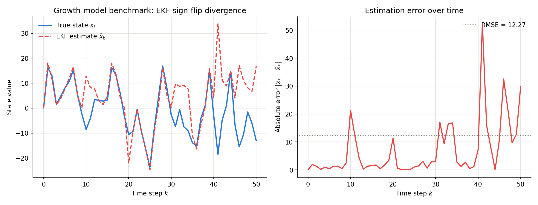
The left panel shows the true state and EKF estimate over time; the right panel shows the absolute error. Errors spike sharply around \(k=10, 20, 31\) -\(34, 41\) — each time the true state either passes near \(x\approx 0\) , where \(h\) ’s curvature is largest, or flips sign. The second-order term \(\mathbf{s}_k\) neglected in Eq. (16) grows with \(h\) ’s nonlinearity and the size of the error, causing the linear approximation to diverge from the actual observation model and the EKF to lose track of the true trajectory.
This benchmark is a one-dimensional scalar system, but as shown in the UKF article , the same mechanism (linearization error proportional to curvature times squared error) appears in multi-dimensional range-bearing tracking too: near the origin, where the observation function’s curvature is largest, the EKF’s error exceeds the UKF’s.
Iterated EKF (IEKF): Improving Accuracy by Iterating the Update
The EKF update in Eqs. (7)-(11) evaluates the observation Jacobian \(\mathbf{H}_k\) at a single point — the predicted state \(\hat{\mathbf{x}}_{k|k-1}\) . But the updated estimate \(\hat{\mathbf{x}}_{k|k}\) generally moves away from \(\hat{\mathbf{x}}_{k|k-1}\) , so evaluating \(\mathbf{H}_k\) at the prediction point is a mismatch relative to the point where it should ideally be evaluated (closer to the true state). The Iterated EKF (IEKF) resolves this mismatch by iterating the update step, progressively refining the linearization point.
The IEKF update step can be written using an iterate \(\boldsymbol{\eta}^{(i)}\) (with \(\boldsymbol{\eta}^{(0)} = \hat{\mathbf{x}}_{k|k-1}\) ):
\[ \mathbf{H}^{(i)} = \frac{\partial h}{\partial \mathbf{x}}\bigg|_{\mathbf{x}=\boldsymbol{\eta}^{(i)}} \tag{19} \] \[ \mathbf{K}^{(i)} = \mathbf{P}_{k|k-1} (\mathbf{H}^{(i)})^T \left[ \mathbf{H}^{(i)} \mathbf{P}_{k|k-1} (\mathbf{H}^{(i)})^T + \mathbf{R} \right]^{-1} \tag{20} \] \[ \boldsymbol{\eta}^{(i+1)} = \hat{\mathbf{x}}_{k|k-1} + \mathbf{K}^{(i)} \Big[ \mathbf{z}_k - h(\boldsymbol{\eta}^{(i)}) - \mathbf{H}^{(i)} \left( \hat{\mathbf{x}}_{k|k-1} - \boldsymbol{\eta}^{(i)} \right) \Big] \tag{21} \]Eq. (21) re-linearizes the observation model around the current iterate \(\boldsymbol{\eta}^{(i)}\) and computes one Gauss-Newton step under that linear approximation. The term \(\mathbf{H}^{(i)}(\hat{\mathbf{x}}_{k|k-1} - \boldsymbol{\eta}^{(i)})\) corrects for the linearization point having drifted from the prediction. Iterating this to convergence (or a fixed number of times) and taking the final \(\hat{\mathbf{x}}_{k|k} = \boldsymbol{\eta}^{(i_{\max})}\) , the covariance is then updated as in the standard EKF using the converged Jacobian. The IEKF is essentially a Gauss-Newton iteration that maximizes the observation log-likelihood, and is known to give more accurate estimates than the standard EKF when \(h\) is strongly nonlinear and the predicted point is far from the true state (truncating at one iteration recovers the plain EKF).
Using the same range-bearing tracking scenario as the UKF and CKF articles (a target approaching to range 1 from the sensor, an initial estimate deliberately far from the truth to simulate re-acquisition, random seed 42), we compare the standard EKF against IEKF (5 iterations). This section is presented as self-contained code (function names match the UKF article ).
import numpy as np

def state_transition(x, dt):
    """State transition function (constant velocity model)"""
    px, py, vx, vy = x
    return np.array([px + vx * dt, py + vy * dt, vx, vy])

def jacobian_F(dt):
    return np.array([
        [1, 0, dt, 0],
        [0, 1, 0, dt],
        [0, 0, 1, 0],
        [0, 0, 0, 1],
    ])

def observation(x):
    """Observation function (range and bearing)"""
    px, py = x[0], x[1]
    r = np.sqrt(px**2 + py**2)
    theta = np.arctan2(py, px)
    return np.array([r, theta])

def jacobian_H(x):
    px, py = x[0], x[1]
    r = np.sqrt(px**2 + py**2)
    return np.array([
        [px / r,      py / r,    0, 0],
        [-py / r**2,  px / r**2, 0, 0],
    ])

def wrap(y):
    """Normalize the bearing residual to [-pi, pi]"""
    y = y.copy()
    y[1] = (y[1] + np.pi) % (2 * np.pi) - np.pi
    return y

# --- Simulation setup (identical to the UKF and CKF articles) ---
np.random.seed(42)
dt = 1.0
T = 80

t = np.arange(0, T + 1) * dt
px_true = np.full(T + 1, 1.0)
py_true = -10.0 + 0.25 * t
true_states = np.column_stack([
    px_true, py_true, np.zeros(T + 1), np.full(T + 1, 0.25)
])

Q = np.diag([0.05, 0.05, 0.01, 0.01])
R = np.diag([0.3, 0.2])

measurements = np.array([
    observation(true_states[k]) + np.random.multivariate_normal([0, 0], R)
    for k in range(1, T + 1)
])

x0 = np.array([6.0, -3.0, 0.0, 0.1])
P0 = np.diag([16.0, 16.0, 1.0, 1.0])
class EKF:
    def __init__(self, x0, P0, Q, R, dt):
        self.x = x0.copy(); self.P = P0.copy()
        self.Q, self.R, self.dt = Q, R, dt

    def predict(self):
        F = jacobian_F(self.dt)
        self.x = state_transition(self.x, self.dt)
        self.P = F @ self.P @ F.T + self.Q

    def update(self, z):
        H = jacobian_H(self.x)
        y = wrap(z - observation(self.x))
        S = H @ self.P @ H.T + self.R
        K = self.P @ H.T @ np.linalg.inv(S)
        self.x = self.x + K @ y
        self.P = (np.eye(4) - K @ H) @ self.P


class IEKF:
    """Iterated EKF: re-evaluates H at the iterate eta within the update step (Eqs. 19-21)"""
    def __init__(self, x0, P0, Q, R, dt, n_iter=5):
        self.x = x0.copy(); self.P = P0.copy()
        self.Q, self.R, self.dt, self.n_iter = Q, R, dt, n_iter

    def predict(self):
        F = jacobian_F(self.dt)
        self.x_pred = state_transition(self.x, self.dt)
        self.P_pred = F @ self.P @ F.T + self.Q
        self.x, self.P = self.x_pred.copy(), self.P_pred

    def update(self, z):
        eta = self.x_pred.copy()
        for _ in range(self.n_iter):
            H = jacobian_H(eta)
            S = H @ self.P_pred @ H.T + self.R
            K = self.P_pred @ H.T @ np.linalg.inv(S)
            innovation = wrap(z - observation(eta)) - H @ (self.x_pred - eta)
            eta = self.x_pred + K @ innovation  # Eq. 21
        self.x = eta
        H = jacobian_H(self.x)
        S = H @ self.P_pred @ H.T + self.R
        K = self.P_pred @ H.T @ np.linalg.inv(S)
        self.P = (np.eye(4) - K @ H) @ self.P_pred
ekf = EKF(x0.copy(), P0.copy(), Q, R, dt)
ekf_estimates = [x0.copy()]
for k in range(T):
    ekf.predict()
    ekf.update(measurements[k].copy())
    ekf_estimates.append(ekf.x.copy())
ekf_estimates = np.array(ekf_estimates)

iekf = IEKF(x0.copy(), P0.copy(), Q, R, dt, n_iter=5)
iekf_estimates = [x0.copy()]
for k in range(T):
    iekf.predict()
    iekf.update(measurements[k].copy())
    iekf_estimates.append(iekf.x.copy())
iekf_estimates = np.array(iekf_estimates)

def rmse(est):
    return np.sqrt(np.mean(
        np.sum((true_states[1:, :2] - est[1:, :2])**2, axis=1)))

print(f"EKF Position RMSE: {rmse(ekf_estimates):.4f}")
print(f"IEKF Position RMSE: {rmse(iekf_estimates):.4f}")
The standard EKF’s RMSE was 1.7155 (reproducing the UKF article ’s number with the same implementation and data), whereas the IEKF with 5 iterations achieved an RMSE of 1.4654 — a roughly 14.6% error reduction over the EKF. Interestingly, this is even smaller than the UKF’s RMSE (1.5489); using 3 iterations instead gives an RMSE of 1.4550 (improvement is limited for 1-2 iterations, plateauing from around 3 onward). This suggests that much of this observation model’s error comes from evaluating the Jacobian at a single, mismatched point, and that IEKF’s iterative re-linearization addresses that mismatch more effectively than the UKF’s sigma-point approximation on this particular problem. That said, note that the UKF and CKF approximate the entire nonlinear transform, including the state transition, whereas the IEKF only improves the linearization point of the observation update (this difference does not show up here because \(f\) happens to be linear in this problem).
Comparing EKF, UKF, and CKF: Accuracy and Computational Cost
The
UKF article
already verified EKF vs. UKF accuracy, and the
CKF article
verified the mathematical equivalence of UKF and CKF, both on the same range-bearing tracking scenario. Here we reuse the same scenario and the state_transition/observation/EKF/Q/R/dt/T/x0/P0/measurements/true_states defined in the previous section, define new UKF and CKF classes, and actually run all three methods to (1) confirm the previously reported accuracy is reproducible, and (2) measure computation time, which neither prior article reported.
import time

class UKF:
    def __init__(self, n, m, f, h, Q, R, alpha=1.0, beta=2, kappa=0):
        self.n, self.m, self.f, self.h = n, m, f, h
        self.Q, self.R = Q, R
        self.lam = alpha**2 * (n + kappa) - n
        self.gamma = np.sqrt(n + self.lam)
        self.Wm = np.full(2 * n + 1, 1 / (2 * (n + self.lam)))
        self.Wc = np.full(2 * n + 1, 1 / (2 * (n + self.lam)))
        self.Wm[0] = self.lam / (n + self.lam)
        self.Wc[0] = self.lam / (n + self.lam) + (1 - alpha**2 + beta)

    def sigma_points(self, x, P):
        L = np.linalg.cholesky(P)
        sigmas = np.zeros((2 * self.n + 1, self.n))
        sigmas[0] = x
        for i in range(self.n):
            sigmas[i + 1] = x + self.gamma * L[:, i]
            sigmas[i + 1 + self.n] = x - self.gamma * L[:, i]
        return sigmas

    def predict(self, x, P, dt):
        sigmas = self.sigma_points(x, P)
        sigmas_pred = np.array([self.f(s, dt) for s in sigmas])
        x_pred = np.dot(self.Wm, sigmas_pred)
        P_pred = self.Q.copy()
        for i in range(2 * self.n + 1):
            d = sigmas_pred[i] - x_pred
            P_pred += self.Wc[i] * np.outer(d, d)
        return x_pred, P_pred, sigmas_pred

    def update(self, x_pred, P_pred, sigmas_pred, z):
        sigmas_z = np.array([self.h(s) for s in sigmas_pred])
        z_pred = np.dot(self.Wm, sigmas_z)
        Pzz = self.R.copy()
        Pxz = np.zeros((self.n, self.m))
        for i in range(2 * self.n + 1):
            dz = wrap(sigmas_z[i] - z_pred)
            dx = sigmas_pred[i] - x_pred
            Pzz += self.Wc[i] * np.outer(dz, dz)
            Pxz += self.Wc[i] * np.outer(dx, dz)
        y = wrap(z - z_pred)
        K = Pxz @ np.linalg.inv(Pzz)
        return x_pred + K @ y, P_pred - K @ Pzz @ K.T


class CKF:
    def __init__(self, n, m, f, h, Q, R):
        self.n, self.m, self.f, self.h = n, m, f, h
        self.Q, self.R = Q, R
        self.w = 1.0 / (2 * n)

    def cubature_points(self, x, P):
        L = np.linalg.cholesky(self.n * P)
        pts = np.zeros((2 * self.n, self.n))
        for i in range(self.n):
            pts[i] = x + L[:, i]
            pts[self.n + i] = x - L[:, i]
        return pts

    def predict(self, x, P, dt):
        X = self.cubature_points(x, P)
        X_pred = np.array([self.f(s, dt) for s in X])
        x_pred = self.w * X_pred.sum(axis=0)
        P_pred = self.Q.copy()
        for i in range(2 * self.n):
            d = X_pred[i] - x_pred
            P_pred += self.w * np.outer(d, d)
        return x_pred, P_pred

    def update(self, x_pred, P_pred, z):
        X = self.cubature_points(x_pred, P_pred)
        Y = np.array([self.h(s) for s in X])
        y_pred = self.w * Y.sum(axis=0)
        S = self.R.copy()
        C = np.zeros((self.n, self.m))
        for i in range(2 * self.n):
            dy = wrap(Y[i] - y_pred)
            dx = X[i] - x_pred
            S += self.w * np.outer(dy, dy)
            C += self.w * np.outer(dx, dy)
        y = wrap(z - y_pred)
        K = C @ np.linalg.inv(S)
        return x_pred + K @ y, P_pred - K @ S @ K.T
def run_ekf():
    ekf = EKF(x0.copy(), P0.copy(), Q, R, dt)
    est = [x0.copy()]
    for k in range(T):
        ekf.predict(); ekf.update(measurements[k].copy())
        est.append(ekf.x.copy())
    return np.array(est)

def run_ukf():
    ukf = UKF(4, 2, state_transition, observation, Q, R)
    x_est, P_est = x0.copy(), P0.copy()
    est = [x_est.copy()]
    for k in range(T):
        x_pred, P_pred, sig = ukf.predict(x_est, P_est, dt)
        x_est, P_est = ukf.update(x_pred, P_pred, sig, measurements[k].copy())
        est.append(x_est.copy())
    return np.array(est)

def run_ckf():
    ckf = CKF(4, 2, state_transition, observation, Q, R)
    x_est, P_est = x0.copy(), P0.copy()
    est = [x_est.copy()]
    for k in range(T):
        x_pred, P_pred = ckf.predict(x_est, P_est, dt)
        x_est, P_est = ckf.update(x_pred, P_pred, measurements[k].copy())
        est.append(x_est.copy())
    return np.array(est)

ekf_est, ukf_est, ckf_est = run_ekf(), run_ukf(), run_ckf()
print(f"EKF RMSE: {rmse(ekf_est):.4f}")
print(f"UKF RMSE: {rmse(ukf_est):.4f}")
print(f"CKF RMSE: {rmse(ckf_est):.4f}")

n_repeat = 200
for name, fn in [("EKF", run_ekf), ("UKF", run_ukf), ("CKF", run_ckf)]:
    t0 = time.perf_counter()
    for _ in range(n_repeat):
        fn()
    t1 = time.perf_counter()
    print(f"{name}: {(t1 - t0) / n_repeat * 1000:.4f} ms/run "
          f"({(t1 - t0) / n_repeat / T * 1e6:.2f} us/step)")
The results (80 steps, random seed 42, averaged over 200 runs) are:
| Method | Position RMSE | Time per run | Time per step |
|---|---|---|---|
| EKF | 1.7155 | 1.40 ms | 17.5 μs |
| UKF | 1.5489 | 9.00 ms | 112.5 μs |
| CKF | 1.5673 | 9.03 ms | 112.8 μs |
The RMSE values — EKF 1.7155 and UKF 1.5489 — match the UKF article ’s numbers exactly, confirming reproducibility. The CKF’s RMSE here is 1.5673, close to but not identical to the UKF’s. As noted in the CKF article , the numerical equivalence between UKF and CKF depends on whether the update step regenerates cubature/sigma points from the predicted covariance or reuses the already-propagated points — a convention we did not align here.
The computation time, however, shows a clear difference: the EKF is about 6.4x faster than the UKF or CKF. This is because the EKF only needs to evaluate the Jacobian once for a state dimension of \(n=4\) , whereas the UKF and CKF must evaluate the nonlinear functions \(f, h\) at \(2n+1=9\) (UKF) or \(2n=8\) (CKF) sigma/cubature points per step, plus a Cholesky decomposition. This confirms, with actual measured time, the theoretical cost ordering shown in the UKF article ’s “Comparison with EKF” table (EKF: \(O(n^2)\) , UKF: \(O(n^3)\) ). Since the accuracy gain from UKF/CKF is under 10% here while the computational cost is more than 6x higher, the EKF can remain a practical choice when nonlinearity is mild or computing resources are constrained, such as real-time estimation on embedded hardware.
Recent Research Trends
The EKF was proposed in the 1960s and is the most classical nonlinear filter, yet its simplicity and low computational cost keep it in wide use for SLAM, autonomous driving, and robot state estimation. A notable recent (2023 onward) research direction is not replacing the EKF but extending it by combining it with neural networks.
Liu, Lai, Bacsa, and Chatzi (2024) propose the “Neural EKF” in “Neural Extended Kalman Filters for Learning and Predicting Dynamics of Structural Systems” (Structural Health Monitoring), parameterizing the state transition and observation functions with neural networks. Unlike conventional variational approaches that train inference and dynamics models as separate networks, the Neural EKF embeds a neural network directly into the EKF’s sequential filtering structure and trains it end-to-end, improving the learning and prediction of complex physical system dynamics such as structures.
Eang and Lee (2024), in “An Integration of Deep Neural Network-Based Extended Kalman Filter (DNN-EKF) Method in Ultra-Wideband (UWB) Localization for Distance Loss Optimization” (Sensors), integrate a DNN with the EKF for indoor robot localization, reporting improved positioning accuracy through reduced UWB ranging error.
What these works share is that they keep the “linearization via Jacobians” framework derived in this article intact, while learning the nonlinear functions \(f, h\) (or a correction term) from data, in effect learning the curvature responsible for linearization error directly from observed data. Even more than half a century after its introduction, and even as the UKF, particle filters, and deep-learning-based methods have become widespread, the EKF continues to be chosen for real-time systems because of its low computational cost — and extending it remains an active area of research.
Related Articles
- Kalman Filter: Theory and Python Implementation - The linear Kalman Filter that EKF extends.
- Unscented Kalman Filter (UKF): Nonlinear State Estimation Theory and Python Implementation - Sigma-point based nonlinear filter that avoids EKF’s linearization.
- Cubature Kalman Filter (CKF): Theory and Python Implementation - Addresses UKF’s weight issues using the spherical-radial cubature rule.
- Particle Filter Python Implementation: Comparing Resampling Methods - A Monte Carlo-based filtering method that handles non-Gaussian distributions.
- Kalman Smoother (RTS Smoother): Theory and Python Implementation - Smoothing using observations from all time steps.
- Kalman Smoother Comparison - Cross-method comparison of Kalman smoothing approaches, including EKF-based nonlinear smoothers.
- Nonlinear Kalman Smoothers (EKS/URTS) - Implements the Extended RTS Smoother using this article’s EKF Jacobian as the backward pass, and compares its accuracy against the UKF-based URTS.
- Filtering Methods in Signal Processing - A systematic overview of KF, EKF, UKF, and particle filters.
- Mathematics of MPPI (Model Predictive Path Integral) - Sampling-based model predictive control that consumes the state estimated by an EKF.
- PID Control in Python: Simulation and Tuning - A canonical feedback controller often paired with EKF-based state estimation.
- Machine Learning Hub for Time-Series, Classification, and Anomaly Detection - Hub article placing EKF alongside linear Kalman, UKF, particle filters, and LSTM as sequential models, organizing their use for anomaly detection and forecasting on nonlinear state spaces.
References
- Thrun, S., Burgard, W., & Fox, D. (2005). “Probabilistic Robotics.” MIT Press.
- Simon, D. (2006). “Optimal State Estimation: Kalman, H-infinity, and Nonlinear Approaches.” Wiley.
- Arulampalam, M. S., Maskell, S., Gordon, N., & Clapp, T. (2002). “A Tutorial on Particle Filters for Online Nonlinear/Non-Gaussian Bayesian Tracking.” IEEE Transactions on Signal Processing, 50(2), 174-188.
- Liu, W., Lai, Z., Bacsa, K., & Chatzi, E. (2024). “Neural Extended Kalman Filters for Learning and Predicting Dynamics of Structural Systems.” Structural Health Monitoring, 23(2), 1037-1052.
- Eang, C., & Lee, S. (2024). “An Integration of Deep Neural Network-Based Extended Kalman Filter (DNN-EKF) Method in Ultra-Wideband (UWB) Localization for Distance Loss Optimization.” Sensors, 24(21), 6959.