What is the Kalman Filter?
The Kalman Filter is an optimal recursive state estimation algorithm for linear Gaussian systems. It sequentially estimates the internal state of a system from noisy observations. Since its introduction by Rudolf E. Kalman in 1960, it has been widely used in navigation, control, signal processing, economics, and many other fields.
The Kalman Filter serves as the foundation for the following extended methods:
- Extended Kalman Filter (EKF) for nonlinear systems
- Unscented Kalman Filter (UKF) based on the Unscented Transform
- Cubature Kalman Filter (CKF)
- Particle Filter
An overview of these methods is available in Basics of Filtering Methods . This article explains the theory and implementation of the most fundamental Kalman Filter.
State-Space Model
The Kalman Filter assumes the following linear state-space model.
State transition model:
\[ \mathbf{x}_k = A \mathbf{x}_{k-1} + B \mathbf{u}_{k-1} + \mathbf{w}_{k-1}, \quad \mathbf{w}_{k-1} \sim \mathcal{N}(\mathbf{0}, Q) \tag{1} \]Observation model:
\[ \mathbf{z}_k = H \mathbf{x}_k + \mathbf{v}_k, \quad \mathbf{v}_k \sim \mathcal{N}(\mathbf{0}, R) \tag{2} \]The variables are defined as follows:
| Symbol | Meaning |
|---|---|
| \(\mathbf{x}_k\) | State vector at time \(k\) |
| \(A\) | State transition matrix |
| \(B\) | Control input matrix |
| \(\mathbf{u}_{k-1}\) | Control input |
| \(\mathbf{w}_{k-1}\) | Process noise (covariance \(Q\) ) |
| \(\mathbf{z}_k\) | Observation vector |
| \(H\) | Observation matrix |
| \(\mathbf{v}_k\) | Observation noise (covariance \(R\) ) |
Algorithm
The Kalman Filter alternates between a prediction step and an update step.
Prediction Step
Predict the current state from the previous estimate.
Predicted state:
\[ \hat{\mathbf{x}}_{k|k-1} = A \hat{\mathbf{x}}_{k-1|k-1} + B \mathbf{u}_{k-1} \tag{3} \]Predicted covariance:
\[ P_{k|k-1} = A P_{k-1|k-1} A^T + Q \tag{4} \]Update Step
Incorporate the new observation to correct the prediction.
Innovation (measurement residual):
\[ \mathbf{y}_k = \mathbf{z}_k - H \hat{\mathbf{x}}_{k|k-1} \tag{5} \]Innovation covariance:
\[ S_k = H P_{k|k-1} H^T + R \tag{6} \]Kalman gain:
\[ K_k = P_{k|k-1} H^T S_k^{-1} \tag{7} \]Updated state:
\[ \hat{\mathbf{x}}_{k|k} = \hat{\mathbf{x}}_{k|k-1} + K_k \mathbf{y}_k \tag{8} \]Updated covariance:
\[ P_{k|k} = (I - K_k H) P_{k|k-1} \tag{9} \]The Kalman gain \(K_k\) automatically adjusts the balance between the prediction and the observation based on their respective uncertainties. When the observation noise is small (\(R\) is small), the filter trusts the observation more. When the process noise is small (\(Q\) is small), the filter trusts the model prediction more.
Deriving the Kalman Gain: Why Is \(K_k\) Optimal?
The previous section handed down the Kalman gain \(K_k = P_{k|k-1} H^T S_k^{-1}\) (Eq. 7) without proof. Here we derive it, showing that this particular \(K_k\) minimizes the trace of the posterior covariance \(\mathrm{tr}(P_{k|k})\) (the sum of the variances of every state component — the MMSE criterion), via two independent routes: (a) direct minimization and (b) the orthogonality principle.
The General Form of the Posterior Error Covariance (Joseph Form)
Treating the gain \(K_k\) as a still-unknown matrix, write the update as
\[ \hat{\mathbf{x}}_{k|k} = \hat{\mathbf{x}}_{k|k-1} + K_k (\mathbf{z}_k - H \hat{\mathbf{x}}_{k|k-1}) \tag{10} \]Expressing the posterior error \(\mathbf{e}_k = \mathbf{x}_k - \hat{\mathbf{x}}_{k|k}\) in terms of the prior error \(\mathbf{e}_k^- = \mathbf{x}_k - \hat{\mathbf{x}}_{k|k-1}\) (covariance \(P_{k|k-1}\) ) and the observation noise \(\mathbf{v}_k\) gives
\[ \mathbf{e}_k = \mathbf{e}_k^- - K_k(H \mathbf{e}_k^- + \mathbf{v}_k) = (I - K_k H)\mathbf{e}_k^- - K_k \mathbf{v}_k \tag{11} \]Since \(\mathbf{e}_k^-\) and \(\mathbf{v}_k\) are uncorrelated (\(\mathbf{v}_k\) is the observation noise at time \(k\) , independent of the earlier estimation error), the cross terms vanish in the covariance and
\[ P_{k|k}(K_k) = (I - K_k H) P_{k|k-1} (I - K_k H)^T + K_k R K_k^T \tag{12} \]This holds for any \(K_k\) , not just the optimal one — it is known as the Joseph stabilized form. Even with rounding error in \(K_k\) , this expression keeps \(P_{k|k}\) symmetric and positive semi-definite, which is why implementations favor it numerically (see the edge cases below).
Deriving the Kalman Gain by Minimizing the Trace
The MMSE criterion is minimizing \(\mathrm{tr}(P_{k|k}(K_k))\) . Expanding Eq. (12) and using the cyclic property of the trace \(\mathrm{tr}(AB)=\mathrm{tr}(BA)\) gives
\[ \mathrm{tr}(P_{k|k}) = \mathrm{tr}(P_{k|k-1}) - 2\,\mathrm{tr}(K_k H P_{k|k-1}) + \mathrm{tr}(K_k S_k K_k^T) \tag{13} \](where \(S_k = H P_{k|k-1} H^T + R\) ). Using the matrix-calculus identities \(\partial\, \mathrm{tr}(K_k H P_{k|k-1})/\partial K_k = P_{k|k-1} H^T\) (since \(P_{k|k-1}\) is symmetric) and \(\partial\, \mathrm{tr}(K_k S_k K_k^T)/\partial K_k = 2 K_k S_k\) (since \(S_k\) is symmetric), differentiate with respect to \(K_k\) and set the result to zero:
\[ \frac{\partial\, \mathrm{tr}(P_{k|k})}{\partial K_k} = -2 P_{k|k-1} H^T + 2 K_k S_k = 0 \tag{14} \]Solving for \(K_k\) recovers exactly Eq. (7):
\[ K_k = P_{k|k-1} H^T S_k^{-1} \tag{15} \]Since \(\partial^2 \mathrm{tr}(P_{k|k})/\partial K_k^2 = 2 S_k \succ 0\) (\(S_k\) is positive definite), this is a genuine minimum, not a saddle point.
Substituting this \(K_k\) back into Eq. (12) and using the normal equation \(K_k S_k = P_{k|k-1}H^T\) ,
\[ P_{k|k} = P_{k|k-1} - K_k H P_{k|k-1} - P_{k|k-1}H^TK_k^T + K_kS_kK_k^T = P_{k|k-1} - K_k H P_{k|k-1} = (I - K_k H)P_{k|k-1} \tag{16} \](substituting \(P_{k|k-1}H^TK_k^T = K_kS_kK_k^T\) cancels the middle two terms), which is exactly the covariance update of Eq. (9).
An Independent Proof via the Orthogonality Principle
A second, equally standard view comes from the general theory of linear MMSE estimation: the orthogonality principle. The error \(\mathbf{e}_k\) of an optimal linear estimator must be uncorrelated with (any linear function of) the observations used to form it. In particular, the innovation \(\mathbf{y}_k\) is “genuinely new information that cannot be predicted from past observations,” so we require \(E[\mathbf{e}_k \mathbf{y}_k^T] = 0\) . From Eq. (11), \(\mathbf{e}_k = \mathbf{e}_k^- - K_k \mathbf{y}_k\) , so
\[ E[\mathbf{e}_k \mathbf{y}_k^T] = E[\mathbf{e}_k^- \mathbf{y}_k^T] - K_k E[\mathbf{y}_k \mathbf{y}_k^T] = P_{k|k-1}H^T - K_k S_k = 0 \tag{17} \](using \(E[\mathbf{e}_k^- \mathbf{y}_k^T] = E[\mathbf{e}_k^-(H\mathbf{e}_k^- + \mathbf{v}_k)^T] = P_{k|k-1}H^T\) and \(E[\mathbf{y}_k\mathbf{y}_k^T]=S_k\) ). Solving gives the same \(K_k = P_{k|k-1}H^T S_k^{-1}\) — confirming that trace minimization and the orthogonality principle produce identical solutions.
Numerical Verification
We confirm the derivation numerically by perturbing the analytical solution in random directions.
import numpy as np

rng = np.random.default_rng(3)

P_minus = np.array([[2.0, 0.5], [0.5, 1.0]])
H = np.array([[1.0, 0.0]])
R = np.array([[0.5]])
S = H @ P_minus @ H.T + R
K_star = P_minus @ H.T @ np.linalg.inv(S)  # analytical solution from Eq. (15)

def trace_P(K):
    """Eq. (12): trace of P_{k|k} in Joseph form"""
    I = np.eye(2)
    P = (I - K @ H) @ P_minus @ (I - K @ H).T + K @ R @ K.T
    return np.trace(P)

print(f"K* (analytical) = {K_star.ravel()}")
print(f"tr(P) at K* = {trace_P(K_star):.6f}")

worse_count = 0
for _ in range(20000):
    dK = rng.normal(scale=0.05, size=K_star.shape)
    if trace_P(K_star + dK) < trace_P(K_star) - 1e-9:
        worse_count += 1
print(f"number of perturbations beating K* (out of 20000): {worse_count}")
Output:
K* (analytical) = [0.8 0.2]
tr(P) at K* = 1.300000
number of perturbations beating K* (out of 20000): 0
Across 20,000 random perturbations of \(K_k\) , none reduces \(\mathrm{tr}(P_{k|k})\) below the value achieved at the analytical solution \(K^*=[0.8,\ 0.2]\) — direct numerical confirmation that Eq. (15) is a local minimum.
Python Implementation
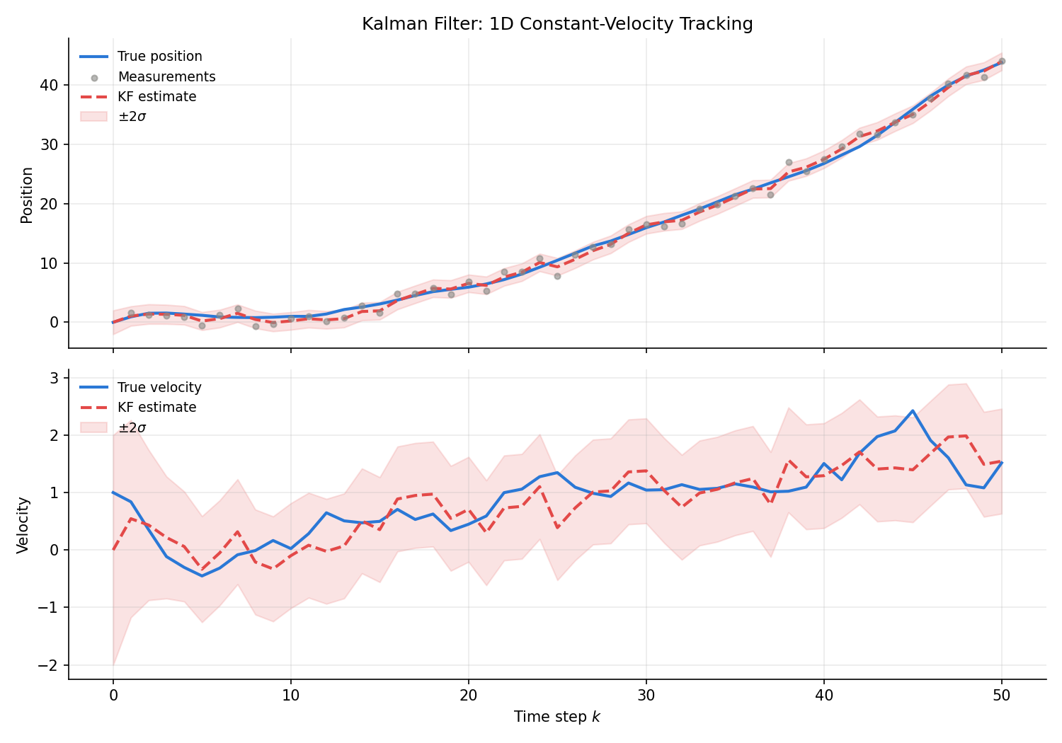
We implement the Kalman Filter using a 1D constant-velocity model.
State-Space Model Definition
The state vector is \(\mathbf{x} = [p, v]^T\) (position, velocity), with the following model:
\[ A = \begin{bmatrix} 1 & \Delta t \\\ 0 & 1 \end{bmatrix}, \quad H = \begin{bmatrix} 1 & 0 \end{bmatrix} \]Only position is observed; velocity is estimated by the filter.
import numpy as np
import matplotlib.pyplot as plt

# ---- Parameter settings ----
dt = 1.0  # time step [s]

# State transition matrix (constant velocity model)
A = np.array([[1, dt],
              [0,  1]])

# Observation matrix (position only)
H = np.array([[1, 0]])

# Process noise covariance (derived from acceleration noise)
q = 0.1  # acceleration noise variance
Q = q * np.array([[dt**3 / 3, dt**2 / 2],
                  [dt**2 / 2, dt]])

# Observation noise covariance
R = np.array([[1.0]])
Kalman Filter Implementation
class KalmanFilter:
    """Linear Kalman Filter"""

    def __init__(self, A, H, Q, R, x0, P0):
        self.A = A
        self.H = H
        self.Q = Q
        self.R = R
        self.x = x0.copy()
        self.P = P0.copy()

    def predict(self, u=None, B=None):
        """Prediction step (Eq. 3, 4)"""
        self.x = self.A @ self.x
        if u is not None and B is not None:
            self.x += B @ u
        self.P = self.A @ self.P @ self.A.T + self.Q
        return self.x.copy(), self.P.copy()

    def update(self, z):
        """Update step (Eq. 5-9)"""
        # Innovation
        y = z - self.H @ self.x
        S = self.H @ self.P @ self.H.T + self.R

        # Kalman gain
        K = self.P @ self.H.T @ np.linalg.inv(S)

        # State and covariance update
        self.x = self.x + K @ y
        I = np.eye(len(self.x))
        self.P = (I - K @ self.H) @ self.P
        return self.x.copy(), self.P.copy()
Simulation
np.random.seed(42)
T = 50  # number of time steps

# True initial state
x_true = np.array([0.0, 1.0])  # position=0, velocity=1

# Kalman Filter initialization
x0 = np.array([0.0, 0.0])     # initial estimate (velocity unknown)
P0 = np.diag([1.0, 1.0])      # initial covariance
kf = KalmanFilter(A, H, Q, R, x0, P0)

# Storage arrays
true_positions = [x_true[0]]
true_velocities = [x_true[1]]
measurements = []
est_positions = [x0[0]]
est_velocities = [x0[1]]
P_history = [P0.copy()]

for k in range(T):
    # True state update
    x_true = A @ x_true + np.random.multivariate_normal([0, 0], Q)
    true_positions.append(x_true[0])
    true_velocities.append(x_true[1])

    # Generate observation
    z = H @ x_true + np.random.multivariate_normal([0], R)
    measurements.append(z[0])

    # Kalman Filter
    kf.predict()
    x_est, P_est = kf.update(z)
    est_positions.append(x_est[0])
    est_velocities.append(x_est[1])
    P_history.append(P_est.copy())

true_positions = np.array(true_positions)
true_velocities = np.array(true_velocities)
measurements = np.array(measurements)
est_positions = np.array(est_positions)
est_velocities = np.array(est_velocities)
P_history = np.array(P_history)

# ---- Plot results ----
time = np.arange(T + 1)
sigma_pos = np.sqrt(P_history[:, 0, 0])

fig, axes = plt.subplots(2, 1, figsize=(12, 8), sharex=True)

# Position estimate
axes[0].plot(time, true_positions, "b-", linewidth=1.5, label="True position")
axes[0].scatter(time[1:], measurements, c="gray", s=15, alpha=0.5,
                label="Measurements", zorder=3)
axes[0].plot(time, est_positions, "r--", linewidth=1.2, label="KF estimate")
axes[0].fill_between(time,
                      est_positions - 2 * sigma_pos,
                      est_positions + 2 * sigma_pos,
                      color="red", alpha=0.15, label="$\pm 2\sigma$")
axes[0].set_ylabel("Position")
axes[0].set_title("Kalman Filter - 1D Constant Velocity Tracking")
axes[0].legend(loc="upper left", fontsize=9)
axes[0].grid(True, alpha=0.3)

# Velocity estimate
sigma_vel = np.sqrt(P_history[:, 1, 1])
axes[1].plot(time, true_velocities, "b-", linewidth=1.5, label="True velocity")
axes[1].plot(time, est_velocities, "r--", linewidth=1.2, label="KF estimate")
axes[1].fill_between(time,
                      est_velocities - 2 * sigma_vel,
                      est_velocities + 2 * sigma_vel,
                      color="red", alpha=0.15, label="$\pm 2\sigma$")
axes[1].set_xlabel("Time step $k$")
axes[1].set_ylabel("Velocity")
axes[1].legend(loc="upper left", fontsize=9)
axes[1].grid(True, alpha=0.3)

plt.tight_layout()
plt.savefig("kalman_filter_result.png", dpi=150)
plt.show()

# RMSE calculation (also compare against the raw, unfiltered observation)
rmse_pos = np.sqrt(np.mean((true_positions[1:] - est_positions[1:]) ** 2))
rmse_meas = np.sqrt(np.mean((true_positions[1:] - measurements) ** 2))
rmse_vel = np.sqrt(np.mean((true_velocities[1:] - est_velocities[1:]) ** 2))
print(f"Position RMSE (KF): {rmse_pos:.4f}")
print(f"Position RMSE (raw measurement): {rmse_meas:.4f}")
print(f"Velocity RMSE (KF): {rmse_vel:.4f}")
print(f"KF position error reduction vs raw measurement: {(1 - rmse_pos/rmse_meas)*100:.1f}%")
Discussion
Running the code above gives a position RMSE of 0.6920 for the KF estimate versus 1.0473 for the raw (unfiltered) observation — a 33.9% error reduction (velocity RMSE is 0.3752). The Kalman Filter converges within a few time steps and accurately estimates the true state from noisy observations. The \(\pm 2\sigma\) confidence band in the figure covers the true state well, indicating that the filter properly quantifies its estimation uncertainty.
Notably, velocity is not directly observed, yet the filter successfully estimates it indirectly from position observations alone. This is a key strength of the Kalman Filter.
Regarding parameter tuning:
- Increasing \(Q\) (process noise): Reduces trust in the model, causing the filter to rely more on observations. This yields faster response but makes estimates noisier.
- Increasing \(R\) (observation noise): Reduces trust in observations, causing the filter to rely more on model predictions. This produces smoother estimates but delays response to actual changes.
The Kalman Filter is limited to linear Gaussian systems. For nonlinear systems, one can use the EKF (Jacobian-based linearization), the UKF or CKF (sigma-point methods), or Particle Filters (Monte Carlo sampling).
Edge Cases and Practical Pitfalls
Even a theoretically perfect Kalman filter needs care in three situations.
Singularity of the Innovation Covariance \(S\)
When \(S_k = H P_{k|k-1}H^T + R\) (Eq. 6) becomes singular or ill-conditioned, computing \(S_k^{-1}\) in Eq. (7) becomes numerically unstable. Common causes are (1) setting the observation noise to exactly \(R=0\) (assuming a perfectly noise-free sensor), and (2) multiple sensors that effectively duplicate the same measured quantity. The following code demonstrates the effect.
import numpy as np

np.random.seed(0)

P_minus = np.array([[1.0, 0.3], [0.3, 0.8]])

# Two "duplicate" sensors that both measure state component 1 (position)
H_dup = np.array([[1.0, 0.0],
                  [1.0, 0.0]])

for r_val, label in [(0.0, "R=0 (duplicate noiseless sensors)"),
                     (1e-10, "R=1e-10 (near-duplicate, tiny noise)"),
                     (1e-2, "R=1e-2 (typical, well-conditioned)")]:
    R_dup = r_val * np.eye(2)
    S = H_dup @ P_minus @ H_dup.T + R_dup
    cond = np.linalg.cond(S)
    print(f"--- {label} ---")
    print(f"cond(S) = {cond:.3e}")
    try:
        K = P_minus @ H_dup.T @ np.linalg.inv(S)
        print("np.linalg.inv(S) succeeded")
    except np.linalg.LinAlgError as e:
        print(f"np.linalg.inv(S) FAILED: {e}")
    K_pinv = P_minus @ H_dup.T @ np.linalg.pinv(S)
    print(f"K via np.linalg.pinv(S) =\n{K_pinv}\n")
Output:
--- R=0 (duplicate noiseless sensors) ---
cond(S) = 1.394e+17
np.linalg.inv(S) FAILED: Singular matrix
K via np.linalg.pinv(S) =
[[0.5  0.5 ]
 [0.15 0.15]]

--- R=1e-10 (near-duplicate, tiny noise) ---
cond(S) = 2.000e+10
K via np.linalg.pinv(S) =
[[0.49999905 0.50000095]
 [0.14999967 0.15000018]]

--- R=1e-2 (typical, well-conditioned) ---
cond(S) = 2.010e+02
K via np.linalg.pinv(S) =
[[0.49751244 0.49751244]
 [0.14925373 0.14925373]]
At \(R=0\)
, the condition number reaches \(\mathrm{cond}(S)\approx1.4\times10^{17}\)
, and np.linalg.inv fails outright with a singular-matrix error (even \(R=10^{-10}\)
still leaves a very ill-conditioned \(\mathrm{cond}(S)=2\times10^{10}\)
). Practical mitigations include:
- Never set the observation noise to exactly zero — add a small regularizing “jitter” floor to \(R\) (e.g., \(10^{-6}\) to \(10^{-9}\) times the expected variance)
- Use
np.linalg.solve(S, ...)instead ofnp.linalg.inv(it avoids explicitly forming the inverse, so it is both faster and more stable) - If duplicate or linearly dependent measurements are known in advance, merge or prune them before the update
- In pathological cases,
np.linalg.pinv(Moore-Penrose pseudo-inverse) returns a minimum-norm solution even for an exactly singular matrix (at the cost of losing the optimality guarantee)
Filter Divergence: Underestimating the Process Noise \(Q\)
Filter divergence is the phenomenon where a Kalman filter becomes overconfident in its own prediction and stops trusting new measurements. A typical cause is configuring the filter with a \(Q\) smaller than the process noise actually present in the true system. If \(P_{k|k-1}=AP_{k-1|k-1}A^T+Q\) (Eq. 4) underestimates \(Q\) , repeated updates drive \(P\) to a value smaller than the actual error, which pushes the Kalman gain \(K_k\) in Eq. (7) toward zero — the filter stops listening to observations almost entirely. This is a positive feedback loop: once divergence starts, it does not self-correct.
The code below sets the true process noise to \(q_\text{true}=0.1\) (the same value used in the main example above), while the filter mistakenly uses \(q_\text{filter}=10^{-6}\) , four orders of magnitude too small.
import numpy as np

np.random.seed(7)

dt = 1.0
A = np.array([[1, dt], [0, 1]])
H = np.array([[1, 0]])

q_true = 0.1
Q_true = q_true * np.array([[dt**3/3, dt**2/2], [dt**2/2, dt]])
R = np.array([[1.0]])

q_filter = 1e-6  # four orders of magnitude too small
Q_filter = q_filter * np.array([[dt**3/3, dt**2/2], [dt**2/2, dt]])

class KalmanFilter:
    def __init__(self, A, H, Q, R, x0, P0):
        self.A, self.H, self.Q, self.R = A, H, Q, R
        self.x, self.P = x0.copy(), P0.copy()

    def predict(self):
        self.x = self.A @ self.x
        self.P = self.A @ self.P @ self.A.T + self.Q
        return self.x.copy(), self.P.copy()

    def update(self, z):
        y = z - self.H @ self.x
        S = self.H @ self.P @ self.H.T + self.R
        K = self.P @ self.H.T @ np.linalg.inv(S)
        self.x = self.x + K @ y
        I = np.eye(len(self.x))
        self.P = (I - K @ self.H) @ self.P
        return self.x.copy(), self.P.copy(), K.copy()

T = 300
x_true = np.array([0.0, 1.0])
kf = KalmanFilter(A, H, Q_filter, R, np.array([0.0, 1.0]), np.diag([1.0, 1.0]))

true_pos, est_pos, P_pos, gains, nees = [x_true[0]], [0.0], [1.0], [], []
for k in range(T):
    x_true = A @ x_true + np.random.multivariate_normal([0, 0], Q_true)
    true_pos.append(x_true[0])
    z = H @ x_true + np.random.multivariate_normal([0], R)
    kf.predict()
    x_est, P_est, K = kf.update(z)
    est_pos.append(x_est[0])
    P_pos.append(P_est[0, 0])
    gains.append(K[0, 0])
    err = (x_true - x_est).reshape(-1, 1)
    nees.append(float((err.T @ np.linalg.inv(P_est) @ err).item()))

true_pos, est_pos, P_pos = np.array(true_pos), np.array(est_pos), np.array(P_pos)
nees = np.array(nees)

print(f"P_pos: k=10 -> {P_pos[10]:.4f}, k=100 -> {P_pos[100]:.4f}, k=299 -> {P_pos[299]:.4f}")
print(f"Kalman gain K_pos: k=10 -> {gains[10]:.4f}, k=100 -> {gains[100]:.4f}, k=299 -> {gains[299]:.4f}")
print(f"mean NEES (last 100 steps): {nees[-100:].mean():.1f} (should be ~1 if consistent; chi2(1) 99% bound is 6.63)")
print(f"RMSE (last 100 steps): {np.sqrt(np.mean((true_pos[-100:]-est_pos[-100:])**2)):.4f}")
print(f"filter-reported sigma (mean over last 100 steps): {np.sqrt(P_pos[-100:]).mean():.4f}")
Output:
P_pos: k=10 -> 0.3161, k=100 -> 0.0469, k=299 -> 0.0437
Kalman gain K_pos: k=10 -> 0.2934, k=100 -> 0.0467, k=299 -> 0.0437
mean NEES (last 100 steps): 48924.8 (should be ~1 if consistent; chi2(1) 99% bound is 6.63)
RMSE (last 100 steps): 11.9092
filter-reported sigma (mean over last 100 steps): 0.2091
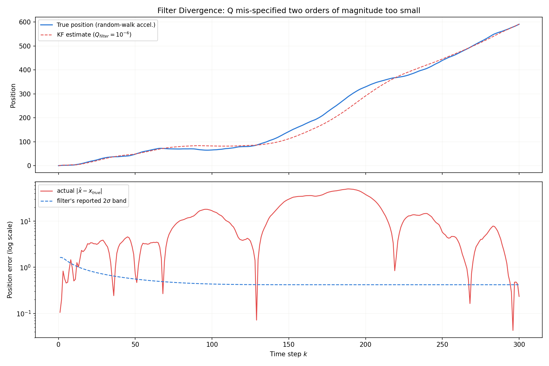
At k=10 the gain is still around 0.29, so the filter is still incorporating observations. From k=100 onward the gain drops to about 0.04 and stays roughly constant, meaning the filter has essentially stopped trusting new measurements. As a result, the standard deviation the filter “confidently” reports stays around 0.21, while the actual RMSE reaches 11.9 — more than 50 times larger — and the mean NEES (normalized estimation error squared, \(\mathbf{e}_k^T P_{k|k}^{-1}\mathbf{e}_k\) ), which should sit near 1 for a consistent filter, blows up to roughly 49,000. This is the textbook signature of divergence: the actual error is large while the reported covariance stays small. Practical mitigations include (1) conservatively overestimating \(Q\) , (2) monitoring consistency online with NEES or an innovation \(\chi^2\) test, (3) using an adaptive Kalman filter that estimates \(Q\) and \(R\) from the data itself, and (4) covariance inflation (a technique commonly used with the Ensemble Kalman Filter ) to artificially inflate \(P\) .
Observability: When a State Component Never Converges
For a Kalman filter to converge to the true state, the system must be observable. For a linear time-invariant system, observability is determined by the rank of the observability matrix
\[ \mathcal{O} = \begin{bmatrix} H \\ HA \\ HA^2 \\ \vdots \\ HA^{n-1} \end{bmatrix} \tag{18} \](\(n\) is the state dimension): the system is observable iff \(\mathrm{rank}(\mathcal{O})=n\) . When \(\mathrm{rank}(\mathcal{O})<n\) , there exist \(n-\mathrm{rank}(\mathcal{O})\) “unobservable directions” whose estimation error never shrinks, no matter how many measurements are collected.
As a concrete example, add a constant sensor bias \(b\) to the position \(p\) and velocity \(v\) state, giving a 3-dimensional system. The observation includes the bias, \(z_k=p_k+b_k+v_k\) — neither \(p\) nor \(b\) alone is observed, only their sum.
import numpy as np

np.random.seed(11)

dt = 1.0
A = np.array([[1, dt, 0], [0, 1, 0], [0, 0, 1]])  # state [p, v, b], b constant
H = np.array([[1, 0, 1]])  # only p + b is observed; neither p nor b alone

O = np.vstack([H @ np.linalg.matrix_power(A, i) for i in range(3)])
rank = np.linalg.matrix_rank(O)
print("Observability matrix O:")
print(O)
print(f"rank(O) = {rank}  (state dimension n=3)")
print("OBSERVABLE" if rank == 3 else "UNOBSERVABLE")
Output:
Observability matrix O:
[[1. 0. 1.]
 [1. 1. 1.]
 [1. 2. 1.]]
rank(O) = 2  (state dimension n=3)
UNOBSERVABLE
\(\mathrm{rank}(\mathcal{O})=2<3\) , so the system is unobservable. Indeed, column 1 (\(p\) ) and column 3 (\(b\) ) of \(O\) are always identical, so the difference direction between \(p\) and \(b\) can never be separated from the observations — only the sum \(p+b\) is informative. Running the filter confirms this.
class KalmanFilter:
    def __init__(self, A, H, Q, R, x0, P0):
        self.A, self.H, self.Q, self.R = A, H, Q, R
        self.x, self.P = x0.copy(), P0.copy()

    def predict(self):
        self.x = self.A @ self.x
        self.P = self.A @ self.P @ self.A.T + self.Q
        return self.x.copy(), self.P.copy()

    def update(self, z):
        y = z - self.H @ self.x
        S = self.H @ self.P @ self.H.T + self.R
        K = self.P @ self.H.T @ np.linalg.inv(S)
        self.x = self.x + K @ y
        I = np.eye(len(self.x))
        self.P = (I - K @ self.H) @ self.P
        return self.x.copy(), self.P.copy()

Q = np.diag([0.01, 0.01, 1e-8])
R = np.array([[0.25]])
x_true = np.array([0.0, 1.0, 2.0])  # true bias b=2.0
kf = KalmanFilter(A, H, Q, R, np.array([0.0, 1.0, 0.0]), np.diag([1.0, 1.0, 4.0]))

P_b_hist, err_b_hist = [], []
for k in range(400):
    x_true = A @ x_true  # noiseless truth, to isolate the observability effect
    z = H @ x_true + np.random.multivariate_normal([0], R)
    kf.predict()
    x_est, P_est = kf.update(z)
    P_b_hist.append(P_est[2, 2])
    err_b_hist.append(x_est[2] - x_true[2])

print(f"P_bias: k=10 -> {P_b_hist[9]:.4f}, k=50 -> {P_b_hist[49]:.4f}, k=399 -> {P_b_hist[398]:.4f}")
print(f"bias estimation error: k=399 -> {err_b_hist[398]:.4f}")
Output:
P_bias: k=10 -> 0.9427, k=50 -> 0.9423, k=399 -> 0.9423
bias estimation error: k=399 -> -0.1808
The bias variance \(P_{bb}\) drops to about 0.94 within the first ~10 steps, but does not decrease at all over the following 389 steps of additional measurements. The bias estimation error also plateaus around \(-0.18\) and never resolves, no matter how much data is collected. Meanwhile, the variance of the observable combination \(p+b\) keeps shrinking monotonically. Both are shown below.
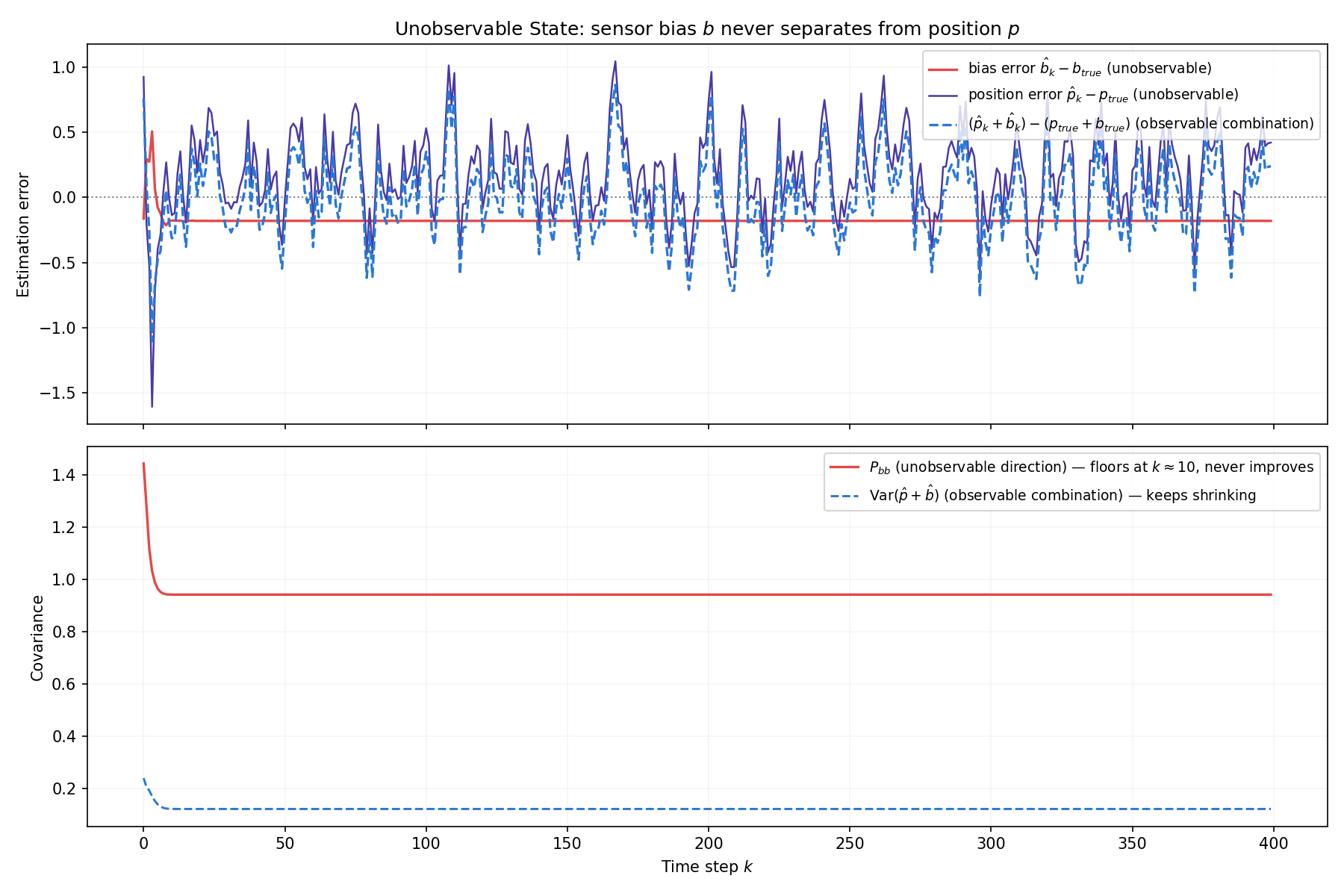
This is a canonical example showing that a correctly implemented filter still fails to converge if the model structure itself is not observable. In practice, designs that deliberately include quantities that cannot be directly observed — accelerometer/gyroscope bias estimation, GPS/INS integrated navigation, and so on — are common, so checking the rank of the observability matrix in advance is recommended. When an unobservable direction exists, mitigations include (1) adding another sensor to raise the rank of \(H\) , (2) removing the unobservable state from the state vector and calibrating it separately, and (3) providing sufficient excitation (e.g., time-varying dynamics, such as commanding motion before estimating the bias) to make the system observable as a time-varying one.
Recent Research Trends
Although the Kalman filter was proposed more than 60 years ago, active research continues on both its theory and its applications.
- Shlezinger, Revach, Ghosh, Chatterjee, Tang, Imbiriba, Dunik, Straka, Closas, & Eldar (2024), “AI-Aided Kalman Filters” (arXiv:2410.12289, revised May 2025), systematically reviews methods (such as KalmanNet) that fuse deep neural networks with the classical Kalman filter when the state-space model is only partially or inaccurately known, categorizing them into task-oriented and model-oriented approaches and summarizing the strengths and limitations of each. A representative approach replaces the Kalman gain \(K_k=P^-H^TS^{-1}\) derived in this article (Eq. 15) with a gain learned by an RNN.
- Mortada, Falcon, Kahil, Clavaud, & Michel (2025), “Recursive KalmanNet: Deep Learning-Augmented Kalman Filtering for State Estimation with Consistent Uncertainty Quantification” (arXiv:2506.11639), incorporates the Joseph-form covariance recursion derived in this article (Eq. 12) into a neural-network training procedure, reporting that it maintains consistent uncertainty (covariance) estimates under non-Gaussian measurement noise while outperforming both classical Kalman filters and prior deep-learning-based approaches.
- Xie, Gan, & Liu (2024), “Stability analysis of distributed Kalman filtering algorithm for stochastic regression model” (arXiv:2411.01198), analyzes the stability of a distributed Kalman filter with no central fusion node under realistic conditions where signals are neither independent nor stationary, and shows conditions under which a quantity that no individual sensor can observe becomes estimable through cooperation among multiple sensors — extending this article’s observability discussion (Eq. 18) to a multi-sensor setting.
All three build on the optimal-gain equation (Eq. 7) and the covariance update (Eq. 9) derived in this article, extending them toward model uncertainty, non-Gaussianity, and distributed systems.
Related Articles
- ARMA/ARIMA in State-Space Form: Kalman-Filter Maximum Likelihood Estimation - Shows ARMA models are a special case of this article’s state-space model, and derives a Kalman-filter likelihood that numerically matches statsmodels’ ARIMA estimation.
- The RLS Algorithm in Python: Recursive Least Squares and Its Equivalence to the Kalman Filter - Numerically demonstrates that the RLS adaptive filter is a special case of the Kalman filter described here.
- Extended Kalman Filter (EKF): Theory and Python Implementation - Extends KF to nonlinear systems using Jacobian-based linearization.
- Fundamentals of Filtering Methods in Signal Processing - Overview of Kalman Filter, EKF, UKF, and Particle Filter.
- Unscented Transformation: Algorithm and Python Implementation - Sigma-point approach to handle nonlinear transformations without linearization.
- Cubature Kalman Filter (CKF): Theory and Python Implementation - Cubature Kalman Filter that resolves the weight issues of UKF.
- Particle Filter Python Implementation: Comparing Resampling Methods - Monte Carlo-based filtering for non-Gaussian distributions.
- Kalman Smoother (RTS Smoother): Theory and Python Implementation - Smooths Kalman Filter results using observations from all time steps.
- Kalman Smoother Comparison - Cross-method comparison of Kalman smoothing approaches, with guidance on choosing a smoother for batch processing.
- Nonlinear Kalman Smoothers in Python: Extended RTS Smoother and Unscented RTS Smoother - Extends this article’s RTS smoother family to nonlinear systems as the backward pass of the EKF and UKF.
- Time-Series Anomaly Detection: From Statistical Methods to Kalman Filter in Python - Innovation-based anomaly detection using the Kalman filter.
- Machine Learning Hub for Time-Series, Classification, and Anomaly Detection - Hub article placing the Kalman filter in the “unsupervised x sequential” cell next to LSTM, GBDT, and Isolation Forest in the broader machine-learning map.
- Ensemble Kalman Filter (EnKF): Theory and Python Implementation - Approximates this article’s update equations using the ensemble’s sample covariance, enabling data assimilation in ultra-high-dimensional systems with a sample count independent of state dimension.
- Anomaly Detection on Prometheus Metrics: EWMA Adaptive Thresholds vs. Kalman Filter in Python - Applies this article’s scalar Kalman filter to anomaly detection on server-monitoring metrics, quantitatively comparing innovation-based thresholding against EWMA.
References
- Welch, G., & Bishop, G. (2006). “An Introduction to the Kalman Filter.” UNC Chapel Hill TR 95-041.
- Thrun, S., Burgard, W., & Fox, D. (2005). “Probabilistic Robotics.” MIT Press.