Fast Fourier Transform (FFT): Theory and Python Implementation with scipy.fft and numpy.fft

Introduction

In signal processing and data analysis, understanding the frequency composition of a signal is critically important. The Fourier Transform decomposes signals into frequency components, and the Discrete Fourier Transform (DFT) applies this concept to discrete data.

However, computing the DFT naively requires \(O(N^2)\) operations, making it impractical for large datasets. The Fast Fourier Transform (FFT) solves this problem by reducing the computational complexity to \(O(N \log N)\) .

This article covers the mathematical definition of the DFT, the mechanics of the FFT algorithm, a from-scratch Python implementation, and practical frequency analysis using NumPy and SciPy.

Discrete Fourier Transform (DFT)

Definition of the DFT

For a discrete signal \(x[n]\) of length \(N\) (\(n = 0, 1, \ldots, N-1\) ), the DFT is defined as:

where:

• \(X[k]\) : the spectrum at frequency index \(k\) (complex-valued)
• \(j\) : the imaginary unit (\(j^2 = -1\) )
• \(e^{-j2\pi kn/N}\) : the twiddle factor

The magnitude \(|X[k]|\) represents the amplitude at each frequency, and the argument \(\angle X[k]\) represents the phase.

Inverse DFT (IDFT)

The inverse transform that recovers the time-domain signal \(x[n]\) from the spectrum \(X[k]\) is:

The DFT and IDFT are invertible, allowing lossless conversion between the time and frequency domains.

Computational Complexity of the DFT

Computing equation \((1)\) directly requires \(N\) complex multiplications and additions for each of the \(N\) values of \(k\) , resulting in \(O(N^2)\) complexity. For \(N = 10^6\) (one million samples), this means \(10^{12}\) operations, which is computationally infeasible.

The FFT Algorithm (Cooley-Tukey Method)

Core Idea

The FFT algorithm, published by Cooley and Tukey in 1965, uses a divide-and-conquer strategy to compute the DFT efficiently. The key idea is to split a length-\(N\) DFT into two length-\(N/2\) DFTs based on even and odd indices.

Separating the input signal \(x[n]\) into even- and odd-indexed samples:

The DFT can then be decomposed as:

Here \(E[k]\) and \(O[k]\) are length-\(N/2\) DFTs of the even and odd subsequences, respectively. Using the twiddle factor \(W_N^k = e^{-j2\pi k/N}\) :

Equation \((6)\) follows from the symmetry property \(W_N^{k+N/2} = -W_N^k\) .

The Butterfly Operation

The pair of equations \((5)\) and \((6)\) is called a butterfly operation. It produces two outputs \((X[k], X[k+N/2])\) from one pair of inputs \((E[k], O[k])\) , named for the shape of its signal flow diagram.

Key properties of the butterfly operation:

• Each butterfly requires one complex multiplication and two complex additions/subtractions
• \(N/2\) butterfly operations form one stage
• Recursive subdivision yields \(\log_2 N\) stages in total

Complexity Reduction

Splitting a length-\(N\) DFT into two length-\(N/2\) DFTs recursively gives the recurrence:

Solving this yields \(T(N) = O(N \log N)\) . For \(N = 10^6\) , this reduces from \(O(N^2) = 10^{12}\) to \(O(N \log N) \approx 2 \times 10^7\) , a speedup of roughly 50,000 times.

Recursive FFT Implementation in Python

To build intuition for the algorithm, here is a recursive implementation in Python. This implementation assumes \(N\) is a power of 2.

import numpy as np

def fft_recursive(x):
    """Recursive FFT implementation (Cooley-Tukey radix-2)"""
    N = len(x)
    if N == 1:
        return x

    # Split into even and odd indices, recurse
    even = fft_recursive(x[0::2])
    odd = fft_recursive(x[1::2])

    # Compute twiddle factors
    T = [np.exp(-2j * np.pi * k / N) * odd[k] for k in range(N // 2)]

    # Butterfly operations
    return [even[k] + T[k] for k in range(N // 2)] + \
           [even[k] - T[k] for k in range(N // 2)]

# Verification: compare with NumPy's FFT
x = np.random.randn(256)
X_custom = np.array(fft_recursive(list(x)))
X_numpy = np.fft.fft(x)
print(f"Max error: {np.max(np.abs(X_custom - X_numpy)):.2e}")
# Example output: Max error: 1.42e-12

While this implementation is useful for understanding the algorithm, the Python list operations introduce significant overhead. For practical use, always use np.fft.fft.

Practical Frequency Analysis with NumPy/SciPy

Basic Usage

NumPy provides the np.fft module for efficient FFT computation.

import numpy as np

# Generate a signal
fs = 1000            # Sampling frequency [Hz]
t = np.arange(0, 1, 1/fs)  # 1 second time axis
signal = np.sin(2 * np.pi * 50 * t)  # 50 Hz sine wave

# Compute FFT
N = len(signal)
X = np.fft.fft(signal)           # Complex spectrum
freqs = np.fft.fftfreq(N, 1/fs)  # Frequency axis [Hz]

np.fft.fftfreq(N, d) returns the frequency values corresponding to each frequency bin. The parameter \(d\) is the sampling interval (\(1/f_s\) ).

Frequency Analysis of a Composite Signal

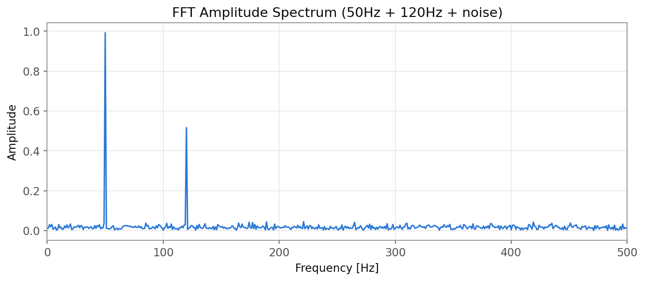
In practice, signals often consist of multiple frequency components with additive noise. The following example visualizes the spectrum of a signal containing 50 Hz and 120 Hz sine waves with Gaussian noise.

import numpy as np
import matplotlib.pyplot as plt

# --- Generate signal ---
np.random.seed(42)
fs = 1000  # Sampling frequency [Hz]
t = np.arange(0, 1, 1/fs)
signal = np.sin(2 * np.pi * 50 * t) + 0.5 * np.sin(2 * np.pi * 120 * t)
signal += 0.3 * np.random.randn(len(t))

# --- FFT ---
N = len(signal)
X = np.fft.fft(signal)
freqs = np.fft.fftfreq(N, 1/fs)

# --- Plot amplitude spectrum (positive frequencies only) ---
plt.figure(figsize=(10, 4))
plt.plot(freqs[:N//2], 2/N * np.abs(X[:N//2]))
plt.xlabel('Frequency [Hz]')
plt.ylabel('Amplitude')
plt.title('FFT Amplitude Spectrum')
plt.grid(True, alpha=0.3)
plt.tight_layout()
plt.show()

The factor 2/N is applied because the FFT output is a two-sided spectrum; when displaying only positive frequencies, the amplitude must be doubled (except for the DC and Nyquist components).

Running the code above produces the following output:

peak near 50Hz: freq=50.0Hz, amplitude=0.9922
peak near 120Hz: freq=120.0Hz, amplitude=0.5163
amplitude ratio (120Hz/50Hz): 0.5204
mean noise-floor amplitude (excluding peaks): 0.0166

The spectrum clearly shows peaks at 50 Hz (amplitude ≈ 0.992) and 120 Hz (amplitude ≈ 0.516), with a ratio of about 0.520 — closely matching the 0.5x amplitude scaling used when the 120 Hz component was added. The noise floor (mean amplitude away from the peaks) is about 0.017, small enough that the two sinusoidal components are cleanly resolved.

Windowing

Spectral Leakage

The FFT implicitly assumes that the finite-length signal is periodic. When the signal is discontinuous at the edges of the analysis window, frequency components that do not actually exist appear in the spectrum. This phenomenon is called spectral leakage.

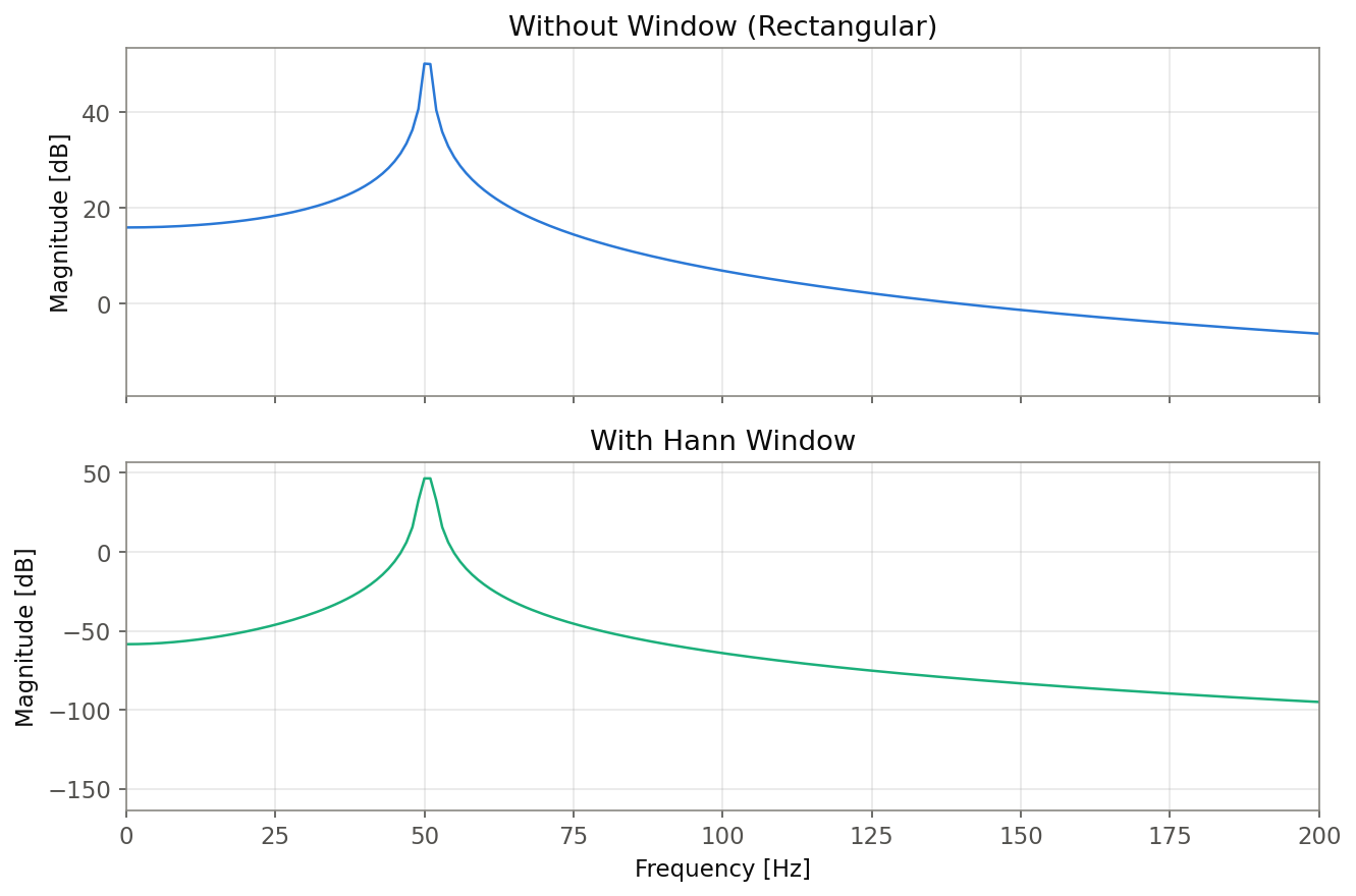
For example, a 50.0 Hz signal sampled at 1000 Hz for exactly 1 second (1000 samples) produces no leakage because the signal completes an integer number of cycles. However, a 50.5 Hz signal creates discontinuities at the window boundaries, causing energy to spread to frequencies other than 50.5 Hz.

Mitigating Leakage with Window Functions

Window functions smoothly taper the signal toward zero at both ends, reducing discontinuities. A commonly used window is the Hann window:

import numpy as np
import matplotlib.pyplot as plt
from scipy.signal.windows import hann

# Signal with spectral leakage (50.5 Hz)
fs = 1000
t = np.arange(0, 1, 1/fs)
signal = np.sin(2 * np.pi * 50.5 * t)
N = len(signal)

# Without window
X_no_win = np.fft.fft(signal)

# With Hann window
window = hann(N)
X_hann = np.fft.fft(signal * window)
freqs = np.fft.fftfreq(N, 1/fs)

# Comparison plot
fig, axes = plt.subplots(2, 1, figsize=(10, 6), sharex=True)

axes[0].plot(freqs[:N//2], 20 * np.log10(np.abs(X_no_win[:N//2]) + 1e-12))
axes[0].set_ylabel('Magnitude [dB]')
axes[0].set_title('Without Window (Rectangular)')
axes[0].set_xlim(0, 200)
axes[0].grid(True, alpha=0.3)

axes[1].plot(freqs[:N//2], 20 * np.log10(np.abs(X_hann[:N//2]) + 1e-12))
axes[1].set_xlabel('Frequency [Hz]')
axes[1].set_ylabel('Magnitude [dB]')
axes[1].set_title('With Hann Window')
axes[1].set_xlim(0, 200)
axes[1].grid(True, alpha=0.3)

plt.tight_layout()
plt.show()

Running the code above produces the following output:

rectangular window: peak=50.0Hz at 50.10dB, max sidelobe (>5Hz away)=28.79dB, main-to-sidelobe gap=21.31dB
hann window: peak=51.0Hz at 46.53dB, max sidelobe (>5Hz away)=-6.10dB, main-to-sidelobe gap=52.63dB

With the rectangular window (no windowing), the main peak reaches 50.10 dB while the largest sidelobe more than 5 Hz away is 28.79 dB — a suppression ratio of only 21.31 dB. Applying the Hann window lowers the main peak somewhat, to 46.53 dB, but pushes the sidelobe (>5 Hz away) down to -6.10 dB, widening the suppression ratio to 52.63 dB. This roughly 31 dB improvement is the quantitative evidence behind “the side lobes are significantly suppressed.” Applying a window function slightly widens the main lobe but significantly suppresses the side lobes, effectively reducing spectral leakage.

Time-Frequency Analysis with STFT

Why STFT Is Needed

A standard FFT computes a single spectrum for the entire signal, losing information about “when” each frequency component was present. For signals whose frequency content changes over time, such as speech or vibration data, the Short-Time Fourier Transform (STFT) is needed.

The STFT segments the signal into short windows and applies the FFT to each segment, producing a time-frequency representation (spectrogram).

where \(L\) is the window length, \(H\) is the hop size (window shift), and \(w[n]\) is the window function.

Chirp Signal Analysis Example

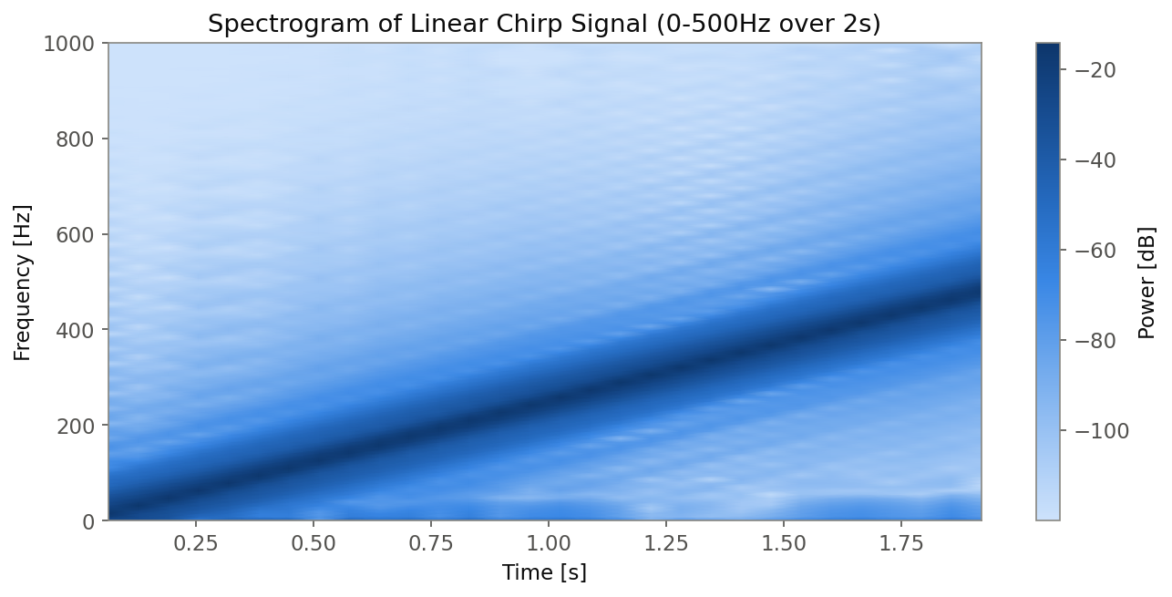
A chirp signal, whose frequency changes linearly over time, is a classic test case for time-frequency analysis.

import numpy as np
import matplotlib.pyplot as plt
from scipy.signal import chirp, spectrogram

# Generate a chirp signal (0 Hz -> 500 Hz over 2 seconds)
fs = 2000  # Sampling frequency [Hz]
t = np.arange(0, 2, 1/fs)
signal = chirp(t, f0=0, f1=500, t1=2, method='linear')

# Compute spectrogram
f, t_spec, Sxx = spectrogram(signal, fs=fs, nperseg=256, noverlap=128)

# Visualization
plt.figure(figsize=(10, 5))
plt.pcolormesh(t_spec, f, 10 * np.log10(Sxx + 1e-12), shading='gouraud')
plt.colorbar(label='Power [dB]')
plt.xlabel('Time [s]')
plt.ylabel('Frequency [Hz]')
plt.title('Spectrogram of Linear Chirp Signal')
plt.tight_layout()
plt.show()

Running the code above produces the following output:

signal length: 4000 samples, duration=2.00s
spectrogram shape: freq_bins=129, time_bins=30
freq resolution: 7.812Hz, time resolution: 0.0640s
tracked peak frequency at t=0.5s: 125.0Hz (expected 125.0Hz)
tracked peak frequency at t=1.0s: 257.8Hz (expected 250.0Hz)
tracked peak frequency at t=1.5s: 367.2Hz (expected 375.0Hz)
mean abs tracking error over all time bins: 1.94Hz

Tracking the frequency bin with maximum power at each time step (an estimate of instantaneous frequency) closely follows the chirp’s theoretical trajectory \(f(t) = 250t\) [Hz], with a mean absolute tracking error of 1.94 Hz across all time bins. This error is mostly attributable to the frequency resolution (7.812 Hz, about half a bin width for nperseg=256); increasing nperseg would sharpen the tracking further, at the cost of the time resolution (currently 0.064 s).

The spectrogram clearly shows the linearly increasing frequency as a diagonal line. Increasing nperseg (window length) improves frequency resolution but reduces time resolution, and vice versa. This is a fundamental trade-off governed by the uncertainty principle.

Recent Research: High-Performance, Fault-Tolerant FFT on GPUs

The theoretical complexity of the FFT (\(O(N \log N)\) ) has not changed since the 1965 Cooley-Tukey algorithm, but optimizing its implementation for GPUs and distributed systems remains an active research area.

A paper submitted in December 2024 and accepted at PPoPP ‘25 (the 30th ACM SIGPLAN Symposium on Principles and Practice of Parallel Programming), “TurboFFT: Co-Designed High-Performance and Fault-Tolerant Fast Fourier Transform on GPUs” (Wu et al., 2024), tackles two problems simultaneously for FFT computation on NVIDIA GPUs:

1. Performance: an architecture-aware, padding-free, template-based design achieves performance comparable to, and in some cases up to 300% faster than, the closed-source cuFFT library on NVIDIA A100 and Tesla T4 GPUs.
2. Reliability: algorithm-based fault tolerance (ABFT) at both the thread and threadblock level detects and corrects computational errors with almost no extra GPU memory, while keeping the performance overhead of fault tolerance to 7-15%.

The np.fft.fft and scipy.fft routines used in this article run on a single CPU core (or a handful of threads), but large-scale scientific computing — weather simulation, astrophysical fluid dynamics, and similar workloads — requires FFTs over billions of points on GPU clusters, where resilience to soft errors (e.g., cosmic-ray-induced bit flips) becomes a real operational concern. Work like TurboFFT shows that even a decades-old, mathematically settled algorithm like the FFT still demands continuous re-engineering at the implementation level as hardware evolves (more GPUs, higher error rates).

Summary

This article covered the definition of the DFT, the mechanics of the Cooley-Tukey FFT algorithm, and practical frequency analysis using NumPy and SciPy.

• DFT decomposes a signal into frequency components with \(O(N^2)\) complexity
• FFT reduces the complexity to \(O(N \log N)\) via divide-and-conquer
• Window functions mitigate spectral leakage
• STFT enables time-frequency analysis for non-stationary signals

The FFT is a cornerstone algorithm in signal processing, with applications spanning filter design, audio analysis, image processing, and telecommunications.

Related Articles

• Frequency Characteristics of the Exponential Moving Average (EMA) Filter - Derives the EMA filter transfer function using the Z-transform and analyzes its frequency response.
• Low-Pass Filter Design and Comparison - Compares moving average, Butterworth, and Chebyshev filter frequency responses using FFT-based methods.
• Moving Average Filters Compared: SMA, WMA, and EMA in Python - Explains the differences in frequency characteristics of SMA, WMA, and EMA.
• Fundamentals of Filtering Methods in Signal Processing - Provides a systematic overview of Kalman filter, EKF, UKF, and particle filter.
• Matplotlib Practical Tips: Creating Publication-Quality Figures - Covers settings for producing higher-quality spectrum plots.
• Window Functions and Power Spectral Density (PSD): Theory and Python Implementation - Detailed window function comparison and Welch’s PSD estimation method.
• Notch Filter Design and Python Implementation - Practical approach to removing specific frequency noise discovered via FFT.
• DTFT, DFT, and FFT: Putting the Hierarchy in Order - A companion article that disentangles the continuous Fourier transform, DTFT, DFT, and FFT and explains zero-padding within that hierarchy.
• Discrete Cosine Transform (DCT): Theory, Fast Computation, and JPEG/Audio Compression - The real-valued member of the Fourier transform family alongside the FFT (DFT); its superior energy compaction underpins JPEG and audio compression.
• Time-Frequency Analysis Guide - An integrated hub that organizes FFT, STFT, wavelet, and Hilbert transforms with a use-case decision flow, situating this article within the broader landscape.

References

• Cooley, J. W., & Tukey, J. W. (1965). “An algorithm for the machine calculation of complex Fourier series”. Mathematics of Computation, 19(90), 297-301.
• Oppenheim, A. V., & Schafer, R. W. (2009). Discrete-Time Signal Processing (3rd ed.). Prentice Hall.
• Wu, S., Zhai, Y., Liu, J., Huang, J., Jian, Z., Dai, H., Di, S., Cappello, F., & Chen, Z. (2024). “TurboFFT: Co-Designed High-Performance and Fault-Tolerant Fast Fourier Transform on GPUs”. PPoPP ‘25. arXiv:2412.05824
• NumPy FFT documentation
• SciPy Signal Processing documentation