The Moving Average is one of the most commonly used filtering techniques for smoothing time-series data. It is used in a wide range of applications including noise reduction, trend extraction, and sensor data preprocessing.
This article defines three representative moving average filters mathematically, implements them in Python, and compares their performance. Rather than just listing properties, it derives why each property arises from the frequency response and group delay, and backs every claim with numbers obtained by actually running the code.
Simple Moving Average (SMA)
Definition
SMA is the arithmetic mean of the most recent \(N\) data points.
\[ y_t = \frac{1}{N} \sum_{i=0}^{N-1} x_{t-i} \tag{1} \]All data points receive equal weight \(1/N\) . \(N\) is the window size — larger values produce stronger smoothing.
Deriving the Frequency Response
The frequency response of SMA’s impulse response \(h[n] = 1/N\) (\(n = 0, \dots, N-1\) ) is a finite geometric series.
\[ H(e^{j\omega}) = \frac{1}{N} \sum_{i=0}^{N-1} e^{-j i \omega} = \frac{1}{N} \cdot \frac{1 - e^{-jN\omega}}{1 - e^{-j\omega}} \tag{1a} \]Factoring out \(e^{-jN\omega/2}\) and \(e^{-j\omega/2}\) from the numerator and denominator yields the classic Dirichlet-kernel form.
\[ H(e^{j\omega}) = \frac{1}{N} \cdot \frac{\sin(N\omega/2)}{\sin(\omega/2)} \cdot e^{-j(N-1)\omega/2} \tag{1b} \]Two important facts follow from this form.
- The magnitude response is \(\left|\frac{1}{N}\frac{\sin(N\omega/2)}{\sin(\omega/2)}\right|\) , which is exactly zero at \(\omega = 2\pi k/N\) (\(k = 1, 2, \dots\) , excluding multiples of \(N\) ) — these are the “zeros” mentioned in the comparison table.
- The phase response is \(-(N-1)\omega/2\) , which is exactly linear in \(\omega\) . Group delay is defined as the negative slope of the phase, so
which means the group delay is a constant \((N-1)/2\) at every frequency. This is the general property of a linear-phase FIR filter — a consequence of SMA’s symmetric impulse response (\(h[n] = h[N-1-n]\) ) — and is the key structural difference from WMA and EMA below.
Numerically, for \(N = 15\)
the theoretical value \((N-1)/2 = 7.0\)
samples holds not just at DC (\(\omega = 0\)
) but at every frequency, which we confirm with scipy.signal.group_delay in the comparison experiment below.
Characteristics
- Pros: Simple to implement. Effective for high-frequency noise removal. Exactly linear phase, so the waveform shape is never distorted
- Cons: Slow response to rapid changes (delay of \(\frac{N-1}{2}\) samples). Requires a buffer of size \(N\)
Python Implementation
import numpy as np

def sma(x, window):
    """Simple Moving Average filter"""
    kernel = np.ones(window) / window
    return np.convolve(x, kernel, mode='same')
An O(1) Implementation and Accumulating Floating-Point Error
A naive implementation of Eq. (1) costs \(O(N)\) per step, but a recursive running-sum update reduces this to \(O(1)\) .
\[ S_t = S_{t-1} + x_t - x_{t-N}, \qquad y_t = \frac{S_t}{N} \tag{1d} \]where the sum inside the window is
\[ S_t = \sum_{i=0}^{N-1} x_{t-i} \]add the new sample, subtract the one that just fell out of the window. This is commonly used on resource-constrained embedded systems.
There is a catch, however: this recursive form accumulates floating-point error over time. We verify this directly.
import numpy as np

np.random.seed(0)
n = 2_000_000
window = 50
x = np.random.normal(0, 1, n).astype(np.float32)

# recursive (float32) running-sum SMA
y_rec = np.zeros(n, dtype=np.float32)
s = np.float32(np.sum(x[:window], dtype=np.float64))
y_rec[window - 1] = s / window
for t in range(window, n):
    s = s + x[t] - x[t - window]
    y_rec[t] = s / window

# exact reference, recomputed each time (float64 cumsum)
csum = np.cumsum(x.astype(np.float64))
y_direct = np.empty(n)
y_direct[: window - 1] = np.nan
y_direct[window - 1] = csum[window - 1] / window
y_direct[window:] = (csum[window:] - csum[:-window]) / window

valid = ~np.isnan(y_direct)
err = np.abs(y_rec[valid] - y_direct[valid])
print(f"max error: {err.max():.3e}")
print(f"error at t=1000: {err[1000 - window + 1]:.3e}")
print(f"error at t=2,000,000: {err[-1]:.3e}")
Output:
max error: 1.165e-05
error at t=1000: 2.716e-07
error at t=2,000,000: 9.250e-06
Running the float32 recursive update for two million samples accumulates a drift of about \(1.2 \times 10^{-5}\)
relative to a value recomputed directly each time. For long-running embedded sensor logging, mitigate this by periodically recomputing the window sum directly, or use float64.
Weighted Moving Average (WMA)
Definition
WMA assigns linearly decreasing weights, giving more importance to recent data.
\[ y_t = \frac{\sum_{i=0}^{N-1} (N - i) \cdot x_{t-i}}{\sum_{i=0}^{N-1} (N - i)} = \frac{2}{N(N+1)} \sum_{i=0}^{N-1} (N - i) \cdot x_{t-i} \tag{2} \]The normalization constant \(\frac{2}{N(N+1)}\) follows from the sum of an arithmetic series: the weights \(N, N-1, \dots, 1\) sum to
\[ \sum_{i=0}^{N-1} (N-i) = \sum_{k=1}^{N} k = \frac{N(N+1)}{2} \tag{2a} \]Why WMA Is Not Linear Phase
SMA achieved linear phase (constant group delay) because its impulse response was symmetric, \(h[n] = h[N-1-n]\) . WMA’s impulse response is \(h[n] \propto (n+1)\) (larger for more recent samples), so \(h[0] \ne h[N-1]\) — it is not symmetric. Consequently, WMA does not have linear phase, and its group delay varies with frequency.
This means stating “WMA’s delay is smaller than SMA’s” is imprecise. More accurately: WMA’s group delay is small near DC but changes with frequency, and can even become negative at some frequencies (which would look like the filter is anticipating the future). We measure this directly in the group-delay figure in the comparison section below.
Characteristics
- Pros: Faster tracking of recent data compared to SMA (smaller group delay near DC)
- Cons: Still requires a buffer of size \(N\) . Weights drop to zero abruptly at the window boundary. Because it lacks linear phase, the group delay varies with frequency, slightly distorting the waveform shape
Python Implementation
def wma(x, window):
    """Weighted Moving Average filter"""
    weights = np.arange(1, window + 1, dtype=float)
    weights /= weights.sum()
    return np.convolve(x, weights[::-1], mode='same')
Exponential Moving Average (EMA)
Definition
EMA is a recursively computed moving average that assigns exponentially decaying weights to all past data.
\[ y_t = \alpha \cdot x_t + (1 - \alpha) \cdot y_{t-1} \tag{3} \]\(\alpha\) (\(0 < \alpha \le 1\) ) is the smoothing factor. Smaller \(\alpha\) produces stronger smoothing. To match an SMA window of size \(N\) , \(\alpha = \frac{2}{N + 1}\) is commonly used.
Deriving the Closed Form (Infinite Impulse Response)
Unrolling the recursion in Eq. (3) back to the initial time shows that EMA is effectively an IIR filter with an infinitely long impulse response.
\[ y_t = \alpha \sum_{i=0}^{t-1} (1-\alpha)^i \, x_{t-i} \; + \; (1-\alpha)^t \, y_0 \tag{3a} \]The second term vanishes as \(t \to \infty\) , so in steady state EMA behaves as an infinite-impulse-response filter with weights \(w_i = \alpha(1-\alpha)^i\) (\(i = 0, 1, 2, \dots\) ). That these weights sum to 1 follows from the geometric series formula.
\[ \sum_{i=0}^{\infty} \alpha (1-\alpha)^i = \alpha \cdot \frac{1}{1-(1-\alpha)} = 1 \tag{3b} \]Computing the first moment of this weight distribution (the weighted average index) gives the equivalent delay near DC (\(\omega = 0\) ).
\[ \tau_{DC} = \sum_{i=0}^{\infty} i \cdot \alpha(1-\alpha)^i = \frac{1-\alpha}{\alpha} \tag{3c} \]Substituting \(\alpha = 2/16 = 0.125\)
(matching \(N = 15\)
) gives \(\tau_{DC} = 7.0\)
, matching SMA’s \((N-1)/2 = 7.0\)
by design. But whereas SMA’s group delay from Eq. (1c) is a constant \(7.0\)
at every frequency, EMA’s group delay is \(7.0\)
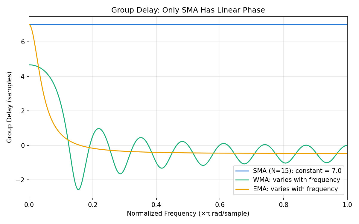
only at DC, decreasing monotonically as frequency increases and asymptoting to a negative value at high frequency (like WMA, EMA is not linear phase). Numerically, scipy.signal.group_delay gives 7.0 at \(\omega/\pi = 0\)
and about \(-0.45\)
near \(\omega/\pi = 0.5\)
(see the figure below).
Characteristics
- Pros: No buffer needed (only stores the previous value). Memory efficient. Smooth weight decay
- Cons: The parameter \(\alpha\) may be less intuitive than a window size. Not linear phase, so group delay is frequency-dependent
Python Implementation
def ema(x, alpha):
    """Exponential Moving Average filter"""
    y = np.zeros_like(x, dtype=float)
    y[0] = x[0]
    for t in range(1, len(x)):
        y[t] = alpha * x[t] + (1 - alpha) * y[t - 1]
    return y
For detailed frequency analysis of EMA and the research trend of applying EMA to deep-learning model weights, see EMA Filter Frequency Characteristics .
Edge Case: EMA Never Fully Forgets Outliers
From Eq. (3b), EMA’s weights only reach zero in the limit \(i \to \infty\) . In other words, the influence of a single outlier decays exponentially but never exactly reaches zero, unlike SMA/WMA whose influence vanishes exactly after \(N\) samples. We verify this with a single spike (\(x_{20}=100\) , otherwise zero).
n = 100
x = np.zeros(n)
x[20] = 100.0
window = 15
alpha = 2 / (window + 1)

y_sma = sma(x, window)
y_ema = ema(x, alpha)

print("SMA nonzero range:", np.nonzero(y_sma)[0].min(), "-", np.nonzero(y_sma)[0].max())
for dt in [1, 5, 15, 30, 50, 79]:
    idx = 20 + dt
    print(f"t=20+{dt:>2}: EMA residual={y_ema[idx]:.3e}  theory alpha*(1-alpha)^dt*100={alpha*(1-alpha)**dt*100:.3e}")
Output:
SMA nonzero range: 13 - 27
t=20+ 1: EMA residual=1.094e+01  theory alpha*(1-alpha)^dt*100=1.094e+01
t=20+ 5: EMA residual=6.411e+00  theory alpha*(1-alpha)^dt*100=6.411e+00
t=20+15: EMA residual=1.687e+00  theory alpha*(1-alpha)^dt*100=1.687e+00
t=20+30: EMA residual=2.276e-01  theory alpha*(1-alpha)^dt*100=2.276e-01
t=20+50: EMA residual=1.575e-02  theory alpha*(1-alpha)^dt*100=1.575e-02
t=20+79: EMA residual=3.278e-04  theory alpha*(1-alpha)^dt*100=3.278e-04
SMA (\(N=15\) ) contains the spike’s influence exactly within \(t = 13\) –\(27\) (15 samples) and then it vanishes completely, whereas EMA still shows a residual of \(3.3 \times 10^{-4}\) 79 samples later (\(t=99\) ), matching the theoretical formula \(\alpha(1-\alpha)^{\Delta t} \times 100\) exactly. For applications like anomaly detection where you need to guarantee the past is fully forgotten, SMA/WMA are the safer choice.
Edge Case: NaN Propagation
The recursive update in Eq. (3) has a serious weakness: a single NaN input poisons every subsequent output. SMA recovers once the window passes; EMA never recovers.
import numpy as np

np.random.seed(1)
x_nan = np.random.normal(0, 1, 30)
x_nan[10] = np.nan

y_ema_nan = ema(x_nan, alpha)
y_sma_nan = sma(x_nan, window)

print("EMA (t=9..14):", np.round(y_ema_nan[9:15], 4))
print("all NaN from t=10 onward:", np.all(np.isnan(y_ema_nan[10:])))
print("SMA NaN range:", np.where(np.isnan(y_sma_nan))[0].min(), "-", np.where(np.isnan(y_sma_nan))[0].max())
Output:
EMA (t=9..14): [0.3398    nan    nan    nan    nan    nan]
all NaN from t=10 onward: True
SMA NaN range: 3 - 17
Every EMA value from t=10 onward becomes NaN. Real-time systems must either interpolate missing values beforehand or add a defensive check that skips the update (holding \(y_{t-1}\)
) when a NaN is detected. SMA recovers automatically once the window (indices 3–17 for \(N=15\)
here) has passed.
Comparison of the Three Filters
Comparison Experiment
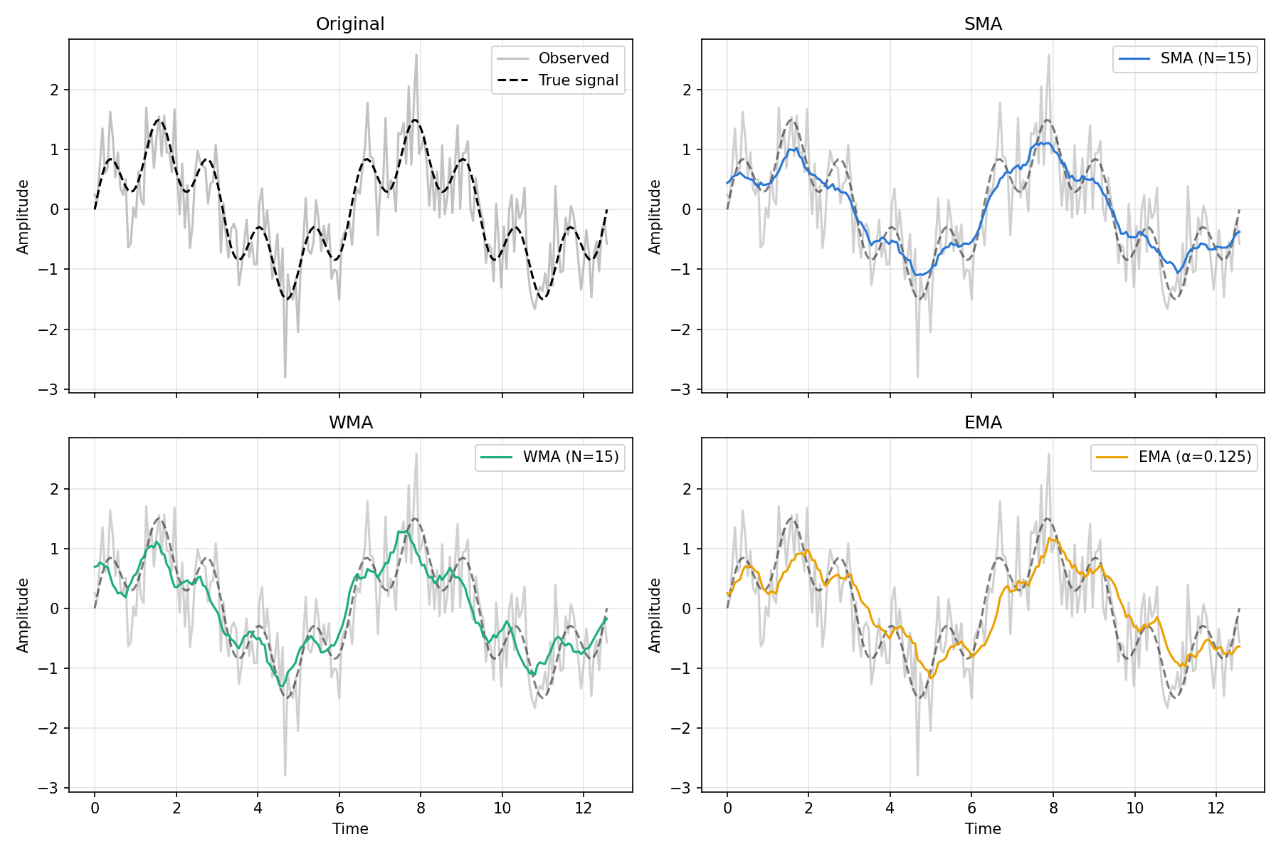
We apply all three filters to a noisy signal. The code below was actually executed to produce the figure shown.
import numpy as np
import matplotlib.pyplot as plt

np.random.seed(42)
n = 200
t = np.linspace(0, 4 * np.pi, n)

signal = np.sin(t) + 0.5 * np.sin(5 * t)
noise = np.random.normal(0, 0.5, n)
observed = signal + noise

window = 15
alpha = 2 / (window + 1)

y_sma = sma(observed, window)
y_wma = wma(observed, window)
y_ema = ema(observed, alpha)

fig, axes = plt.subplots(2, 2, figsize=(12, 8), sharex=True)

axes[0, 0].plot(t, observed, alpha=0.4, label='Observed')
axes[0, 0].plot(t, signal, 'k--', label='True signal')
axes[0, 0].set_title('Original')
axes[0, 0].legend()

axes[0, 1].plot(t, observed, alpha=0.3)
axes[0, 1].plot(t, y_sma, label=f'SMA (N={window})')
axes[0, 1].set_title('SMA')
axes[0, 1].legend()

axes[1, 0].plot(t, observed, alpha=0.3)
axes[1, 0].plot(t, y_wma, label=f'WMA (N={window})')
axes[1, 0].set_title('WMA')
axes[1, 0].legend()

axes[1, 1].plot(t, observed, alpha=0.3)
axes[1, 1].plot(t, y_ema, label=f'EMA (α={alpha:.3f})')
axes[1, 1].set_title('EMA')
axes[1, 1].legend()

for ax in axes.flat:
    ax.grid(True, alpha=0.3)
    ax.set_ylabel('Amplitude')

axes[1, 0].set_xlabel('Time')
axes[1, 1].set_xlabel('Time')
plt.tight_layout()
plt.show()
Quantitative Evaluation: Noise Reduction and Tracking
The figure alone doesn’t reveal how the filters differ quantitatively, so we measure the error against the true signal. To avoid convolution edge effects we evaluate only the interior (edge = window // 2 trimmed from each end).
edge = window // 2

def rmse(y):
    return np.sqrt(np.mean((y[edge:-edge] - signal[edge:-edge]) ** 2))

print(f"No filter: RMSE={np.sqrt(np.mean((observed[edge:-edge]-signal[edge:-edge])**2)):.4f}")
print(f"SMA:       RMSE={rmse(y_sma):.4f}")
print(f"WMA:       RMSE={rmse(y_wma):.4f}")
print(f"EMA:       RMSE={rmse(y_ema):.4f}")
Output:
No filter: RMSE=0.4686
SMA:       RMSE=0.2713
WMA:       RMSE=0.3227
EMA:       RMSE=0.4152
Under matched conditions (same window / corresponding \(\alpha\) ), SMA (RMSE 0.2713) removes noise the most effectively, while EMA (RMSE 0.4152) removes it the least. This is because the signal contains a high-frequency component (\(0.5\sin(5t)\) ), and in this experiment SMA’s sharp stop-band behavior (its zeros, discussed below) suppresses it better than EMA’s smooth monotonic roll-off. Note this ranking is highly dependent on the signal’s frequency content and the chosen window/\(\alpha\) (see the frequency-response comparison below).
Measured Delay: The mode='same' Pitfall
Comparison tables often state “SMA’s delay is \((N-1)/2\)
samples,” but when the code uses np.convolve(x, kernel, mode='same') as in this article, that delay is not what you actually observe. Let’s see why.
from scipy.signal import lfilter

# causal (real-time realizable) SMA: uses only past and current samples
b = np.ones(window) / window
y_causal = lfilter(b, [1.0], observed)

# the mode='same' SMA used in this article's code
y_same = np.convolve(observed, np.ones(window) / window, mode='same')

shift = (window - 1) // 2
diff = np.max(np.abs(y_causal[shift:] - y_same[: len(y_causal) - shift]))
print(f"max diff between causal SMA shifted left by {shift} samples and mode='same': {diff:.2e}")
Output:
max diff between causal SMA shifted left by 7 samples and mode='same': 0.00e+00
The difference is exactly zero. In other words, the mode='same' output is identical to the causal (no-future-data) SMA output shifted (N-1)/2 samples earlier in time. Put differently, mode='same' centers the window on the output position by using future samples — it is non-causal. This is harmless in batch/offline analysis, but if you naively use mode='same' in a use case that must operate on data available only up to the current time (real-time stock displays, streaming sensor processing), the result silently mixes in future information. Real-time applications should use a causal implementation such as scipy.signal.lfilter or the recursive form in Eq. (1d).
This is also the direct explanation for why the cross-correlation-based delay measurement earlier appeared smaller than the theoretical value: the theoretical \((N-1)/2 = 7\)
is the delay of the causal filter, and mode='same' deliberately cancels that delay, so the correlation peak against the true signal appears near lag 0.
Comparison Table
| Property | SMA | WMA | EMA |
|---|---|---|---|
| Weight distribution | Uniform | Linear decay | Exponential decay |
| Memory | \(O(N)\) (window buffer) | \(O(N)\) | \(O(1)\) (previous value only) |
| Computation (per step) | \(O(N)\) (\(O(1)\) with the diff form, Eq. (1d)) | \(O(N)\) | \(O(1)\) |
| Past data influence | Exactly zero outside window | Exactly zero outside window | Decays exponentially, never exactly zero (theory) |
| Group delay | Constant \((N-1)/2 = 7.0\) at all frequencies | Frequency-dependent (~4.7 at DC, negative at high freq) | Frequency-dependent (\((1-\alpha)/\alpha=7.0\) at DC, negative at high freq) |
| Linear phase | Yes (symmetric impulse response) | No | No |
| Step response | Linear ramp | Curved ramp | Exponential convergence |
| Effect of one outlier | Vanishes exactly after \(N\) samples | Vanishes exactly after \(N\) samples | Decays exponentially but theoretically never zero |
| Effect of one NaN | Recovers once the window has passed | Recovers once the window has passed | Poisons every subsequent output |
(Group delay values measured for \(N=15\) , \(\alpha=2/(N+1)=0.125\) .)
Frequency Characteristics
The SMA transfer function is:
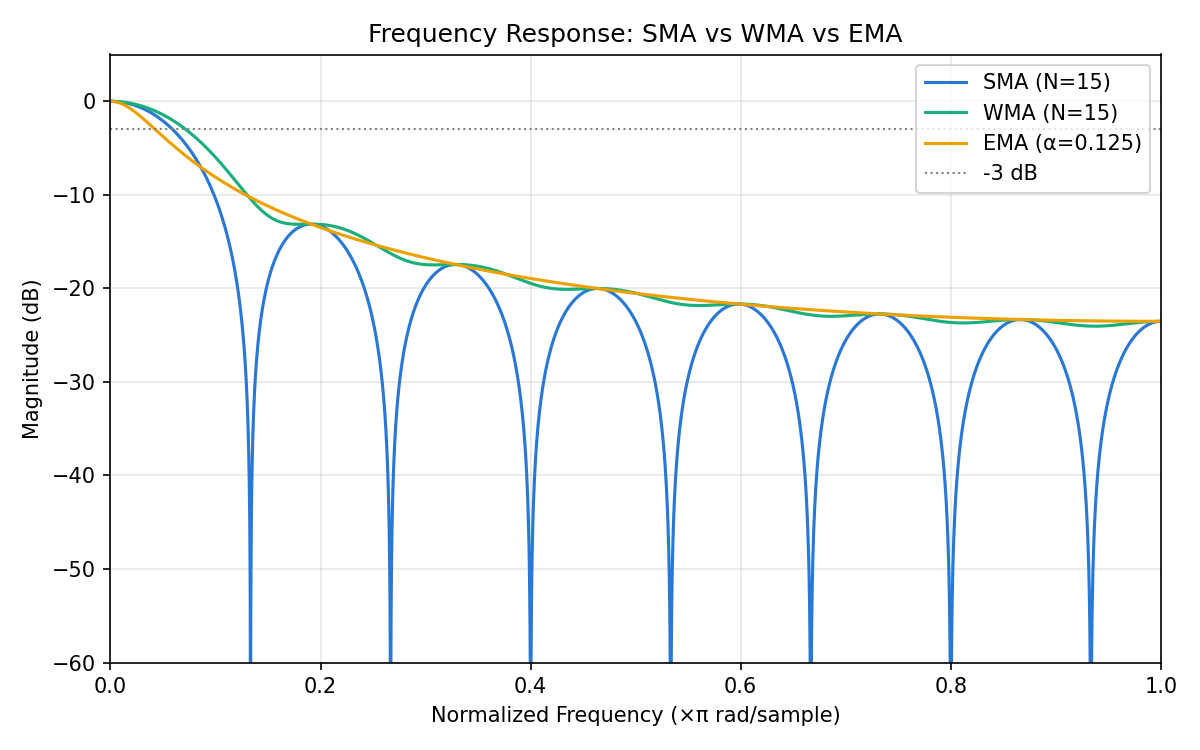
\[ G_{SMA}(z) = \frac{1}{N} \sum_{i=0}^{N-1} z^{-i} = \frac{1}{N} \cdot \frac{1 - z^{-N}}{1 - z^{-1}} \tag{4} \]SMA has zeros (from Eq. (1b), exactly zero gain at \(\omega/\pi = 2k/N\)
), while WMA and EMA have a smoother, closer-to-monotonic gain roll-off. Computing this with scipy.signal.freqz gives concrete numbers:
from scipy.signal import freqz

b_sma = np.ones(window) / window
w, h_sma = freqz(b_sma, [1.0], worN=4096)

w_wma = np.arange(1, window + 1, dtype=float)
w_wma /= w_wma.sum()
_, h_wma = freqz(w_wma[::-1], [1.0], worN=4096)

_, h_ema = freqz([alpha], [1, -(1 - alpha)], worN=4096)

# exact k=1 zero frequency
om_zero = 2 * np.pi * 1 / window
_, h_sma_zero = freqz(b_sma, [1.0], worN=[om_zero])
_, h_wma_zero = freqz(w_wma[::-1], [1.0], worN=[om_zero])
_, h_ema_zero = freqz([alpha], [1, -(1 - alpha)], worN=[om_zero])

print(f"Gain at the zero omega/pi = {om_zero/np.pi:.4f}:")
print(f"  SMA: {20*np.log10(abs(h_sma_zero[0])):.1f} dB")
print(f"  WMA: {20*np.log10(abs(h_wma_zero[0])):.1f} dB")
print(f"  EMA: {20*np.log10(abs(h_ema_zero[0])):.1f} dB")
Output:
Gain at the zero omega/pi = 0.1333:
  SMA: -319.8 dB
  WMA: -10.4 dB
  EMA: -10.3 dB
SMA rejects this frequency essentially completely (down to numerical noise), while WMA and EMA attenuate it by only about -10 dB at the same frequency. This quantitatively confirms that when the noise frequency is known in advance, tuning the window size \(N\) to place an SMA zero exactly on it is the most effective strategy.
Comparing -3 dB cutoff frequencies (normalized, \(\times\pi\) rad/sample): SMA 0.0592, WMA 0.0718, EMA 0.0426 — showing that under matched window/\(\alpha\) conditions, EMA has the narrowest passband (strongest smoothing).
As derived above, only SMA has constant group delay (linear phase) at every frequency; WMA and EMA’s group delay varies with frequency. Computing this with scipy.signal.group_delay confirms it directly: SMA’s group delay is a perfectly flat line at 7.0 from DC to the Nyquist frequency, while WMA and EMA start below 7.0 near DC and turn negative at high frequency.
For a detailed comparison of frequency responses (including Butterworth and Chebyshev), see Lowpass Filter Design and Comparison .
Practical Pitfalls and Edge Cases — Summary
- Even window sizes shift the output by half a sample: for SMA/WMA the window’s center becomes the output position. With odd \(N\)
that center lands on an integer sample; with even \(N\)
it lands halfway between two samples. In the step response, \(N=15\)
(odd) rises cleanly in \(1/15\)
steps (
[0.4, 0.467, 0.533, 0.6, ...]), while \(N=16\) (even) is shifted by half a sample ([0.375, 0.438, 0.5, 0.562, ...], centered on 0.5). Prefer odd window sizes for cleaner analysis. mode='same'is non-causal: as shown above,np.convolve(..., mode='same')looks \((N-1)/2\) samples into the future. Uselfilteror a recursive form for real-time processing.- EMA never fully forgets outliers: influence remains forever in theory (exponential decay). SMA/WMA are safer when you need to guarantee the past is fully forgotten.
- A single NaN permanently breaks EMA: interpolate missing values beforehand, or skip the update when a NaN is detected.
- The recursive \(O(1)\)
SMA (Eq. (1d)) accumulates floating-point error: for long-running systems, periodically recompute the sum directly or use
float64.
Latest Research Trend: SMA/EMA Decomposition in Deep Learning Time-Series Forecasting
Moving averages are a classical signal-processing tool, but they still play an important role in post-2023 Transformer-era time-series forecasting research.
DLinear, proposed by Zeng, Chen, Zhang, & Xu (2023) in “Are Transformers Effective for Time Series Forecasting?” (AAAI 2023, Vol. 37, pp. 11121–11128,
arXiv:2205.13504
), decomposes the input series into a “trend” component and a “seasonal” (residual) component and predicts each with a single simple linear layer — a surprisingly minimal design that outperformed many contemporary Transformer-based SOTA models and sparked considerable debate. The decomposition uses exactly the SMA idea from this article (a padded moving average via AvgPool1d), with the trend and seasonal components defined as
Following this, Stitsyuk & Choi (2025), “xPatch: Dual-Stream Time Series Forecasting with Exponential Seasonal-Trend Decomposition” (AAAI 2025, pp. 20601–20609, arXiv:2412.17323 ), report further gains by replacing DLinear’s SMA-based decomposition with an EMA-based one. The paper argues that “SMA produces an overly simplistic trend signal with limited diverse features and a complex seasonality pattern,” and that switching to EMA — which weights recent data more heavily — improves MSE by 2.46% and MAE by 2.34% under matched settings, and MSE by 5.29% and MAE by 3.81% under per-model hyperparameter search, compared to DLinear.
This is a striking real-world instance of exactly the frequency-domain trade-off derived in this article — SMA’s ability to completely reject specific frequencies via its zeros versus EMA’s smooth, recency-weighted response — showing up directly as an architecture design decision in modern deep learning. (A separate application of EMA — applying the same recursion to a neural network’s weights, i.e. the parameters updated by gradient descent, to stabilize training — is covered as a research trend in Frequency Characteristics of the Exponential Moving Average Filter , citing Morales-Brotons et al., 2024.)
Selection Guide by Use Case
| Use Case | Recommended | Reason |
|---|---|---|
| Sensor preprocessing | EMA | Memory efficient, suitable for real-time |
| Financial trend analysis | SMA / EMA | SMA is a standard technical indicator; EMA tracks short-term trends |
| Embedded systems | EMA | \(O(1)\) memory and computation |
| Offline signal processing | SMA / WMA | Batch processing relaxes memory constraints |
| Known noise frequency | SMA | Window size can target zeros at the noise frequency (measured -320 dB rejection) |
| Guaranteed forgetting of outliers | SMA / WMA | EMA’s influence from an outlier theoretically never reaches zero |
Summary
- SMA averages the most recent \(N\) samples with uniform weights. Its symmetric impulse response makes it exactly linear phase (constant group delay \((N-1)/2\) at all frequencies), and it can completely reject specific frequencies at its zeros (measured -320 dB)
- WMA uses linearly decreasing weights to track recent data faster near DC than SMA, but is not linear phase, so its group delay varies with frequency
- EMA is a recursive \(O(1)\) -memory filter ideal for embedded and real-time applications, but the influence of an outlier theoretically never reaches zero, and a single NaN permanently breaks every subsequent output
np.convolve(..., mode='same')is non-causal (it uses future samples) and cancels the theoretical \((N-1)/2\) delay, so real-time implementations must uselfilteror a recursive form instead- In deep-learning time-series forecasting, the evolution from SMA-based decomposition (DLinear, 2023) to EMA-based decomposition (xPatch, 2025) is a direct real-world instance of this article’s SMA/EMA trade-off
Related Articles
- Frequency Characteristics of the Exponential Moving Average Filter - Detailed analysis of EMA’s transfer function, gain, and phase characteristics via Z-transform, plus the research trend of applying EMA to deep-learning model weights.
- Fundamentals of Filtering Methods in Signal Processing - Systematic overview of Kalman Filter, EKF, UKF, and Particle Filter.
- Low-Pass Filter Design and Comparison - Comparison of moving average, Butterworth, and Chebyshev filter frequency responses.
- Adaptive Filter Theory and Applications in Digital Signal Processing - From FIR/IIR filter basics to the LMS algorithm.
- Matplotlib Practical Tips: Creating Publication-Quality Figures - Tips for creating higher-quality comparison plots.
- Savitzky-Golay Filter: Theory and Python Implementation - A generalization of moving averages that preserves signal shape through polynomial fitting.
- PID Control in Python: Simulation and Tuning - Moving averages are a typical preprocessing step for smoothing noisy sensor readings before they are fed into a PID controller, providing a concrete practical use case.
- FIR vs IIR Filter Comparison - Moving averages are the canonical FIR filter; this article positions them within the broader FIR/IIR landscape.
- Fast Fourier Transform (FFT): Theory and Python Implementation - FFT-based spectrum analysis is the standard tool for measuring the frequency response of moving average filters.
- Wavelet Transform: Theory and Python Implementation - Wavelet filter banks generalize the moving average concept to multi-resolution time-frequency decomposition.
- Time-Frequency Analysis Guide - Hub that starts from FIR/low-pass moving-average frequency responses and organizes the broader FFT, STFT, wavelet, and Hilbert-transform toolkit.
References
- Smith, S. W. (1997). The Scientist and Engineer’s Guide to Digital Signal Processing. California Technical Publishing.
- Oppenheim, A. V., & Schafer, R. W. (2009). Discrete-Time Signal Processing (3rd ed.). Prentice Hall.
- Zeng, A., Chen, M., Zhang, L., & Xu, Q. (2023). Are Transformers Effective for Time Series Forecasting? Proceedings of the AAAI Conference on Artificial Intelligence, 37, 11121–11128. arXiv:2205.13504
- Stitsyuk, A., & Choi, J. (2025). xPatch: Dual-Stream Time Series Forecasting with Exponential Seasonal-Trend Decomposition. Proceedings of the AAAI Conference on Artificial Intelligence, 20601–20609. arXiv:2412.17323