Introduction
PID control is the most widely used feedback control method in industry. It appears in temperature control, motor control, process control, and countless other applications.
For the theoretical foundations of PID control, see Fundamentals of PID Control and the Role of Each Component . In this article, we implement a PID controller in Python, simulate its behavior with a first-order system, compare P/PI/PID step responses, and introduce the classical Ziegler-Nichols tuning method.
Implementing a Discrete PID Controller
The continuous-time PID control law is expressed as:
\[ u(t) = K_P e(t) + K_I \int_0^t e(\tau)d\tau + K_D \frac{de(t)}{dt} \]where \(e(t) = r(t) - y(t)\) is the error between the setpoint and the output. For computer implementation, we approximate the integral with a cumulative sum and the derivative with a backward difference, yielding the discrete PID control law:
\[ u[k] = K_P e[k] + K_I \Delta t \sum_{i=0}^{k} e[i] + K_D \frac{e[k] - e[k-1]}{\Delta t} \tag{1} \]where \(\Delta t\) is the sampling period.
The following Python implementation includes output limiting and anti-windup.
class PIDController:
    def __init__(self, kp, ki, kd, dt, output_limits=None):
        self.kp = kp
        self.ki = ki
        self.kd = kd
        self.dt = dt
        self.output_limits = output_limits
        self.integral = 0.0
        self.prev_error = 0.0

    def update(self, setpoint, measured):
        error = setpoint - measured

        # Proportional term
        p_term = self.kp * error

        # Integral term (cumulative sum approximation)
        self.integral += error * self.dt
        i_term = self.ki * self.integral

        # Derivative term (backward difference approximation)
        derivative = (error - self.prev_error) / self.dt
        d_term = self.kd * derivative
        self.prev_error = error

        output = p_term + i_term + d_term

        # Output limiting (anti-windup)
        if self.output_limits is not None:
            lo, hi = self.output_limits
            if output > hi:
                output = hi
                self.integral -= error * self.dt
            elif output < lo:
                output = lo
                self.integral -= error * self.dt

        return output

    def reset(self):
        self.integral = 0.0
        self.prev_error = 0.0
The anti-windup mechanism stops the integral term from accumulating when the output reaches its limits. Without it, the integral value would grow unboundedly during saturation, causing a large overshoot when the constraint is released.
Plant Model
We use a first-order system as the plant for simulation. Its transfer function is:
\[ G(s) = \frac{K}{1 + Ts} \tag{2} \]where \(K\) is the process gain and \(T\) is the time constant. Discretizing this differential equation gives the following update rule:
\[ y[k+1] = y[k] + \frac{\Delta t}{T}(K \cdot u[k] - y[k]) \tag{3} \]The Python implementation is as follows.
class FirstOrderSystem:
    def __init__(self, gain, time_constant, dt):
        self.gain = gain
        self.time_constant = time_constant
        self.dt = dt
        self.y = 0.0

    def update(self, u):
        self.y += self.dt / self.time_constant * (self.gain * u - self.y)
        return self.y

    def reset(self):
        self.y = 0.0
Comparing P, PI, and PID Step Responses
We compare the step responses of three controller types. The plant has \(K=1.0\) and \(T=1.0\) .
import numpy as np
import matplotlib.pyplot as plt

dt = 0.01
t_end = 10.0
t = np.arange(0, t_end, dt)
setpoint = np.ones_like(t)  # Step input

plant_params = {'gain': 1.0, 'time_constant': 1.0, 'dt': dt}

configs = [
    ('P control (Kp=2.0)', {'kp': 2.0, 'ki': 0.0, 'kd': 0.0}),
    ('PI control (Kp=2.0, Ki=1.0)', {'kp': 2.0, 'ki': 1.0, 'kd': 0.0}),
    ('PID control (Kp=2.0, Ki=1.0, Kd=0.5)', {'kp': 2.0, 'ki': 1.0, 'kd': 0.5}),
]

fig, axes = plt.subplots(2, 1, figsize=(10, 8), sharex=True)

for label, params in configs:
    pid = PIDController(**params, dt=dt)
    plant = FirstOrderSystem(**plant_params)
    y_hist = []
    u_hist = []

    for sp in setpoint:
        u = pid.update(sp, plant.y)
        y = plant.update(u)
        y_hist.append(y)
        u_hist.append(u)

    axes[0].plot(t, y_hist, label=label)
    axes[1].plot(t, u_hist, label=label)

axes[0].axhline(y=1.0, color='k', linestyle='--', alpha=0.5, label='Setpoint')
axes[0].set_ylabel('Output y(t)')
axes[0].set_title('Step Response Comparison')
axes[0].legend()
axes[0].grid(True, alpha=0.3)

axes[1].set_ylabel('Control input u(t)')
axes[1].set_xlabel('Time [s]')
axes[1].legend()
axes[1].grid(True, alpha=0.3)

plt.tight_layout()
plt.show()
From the simulation results, the following characteristics can be observed:
- P control: The response is fast, but a steady-state error remains. With \(K_P = 2.0\) , the theoretical steady-state error is \(\frac{1}{1 + K \cdot K_P} = \frac{1}{3} \approx 0.33\) .
- PI control: The integral term eliminates the steady-state error. However, overshoot tends to increase.
- PID control: The derivative term suppresses overshoot, achieving both the fast response of P control and the steady-state accuracy of PI control.
Effect of Gain Parameters
The setting of each gain parameter significantly affects control performance.
Excessive Proportional Gain \(K_P\)
Setting \(K_P\) too large makes the response oscillatory and eventually unstable. For example, with P control at \(K_P = 10.0\) , the output oscillates around the setpoint.
Integral Gain \(K_I\) and Windup
When \(K_I\) is large or the control output is constrained, the integral term can accumulate excessively, a phenomenon called “windup.” While the output is saturated, the integral value keeps growing, causing a large overshoot after the constraint is released. The anti-windup mechanism described earlier mitigates this problem. The mechanism behind windup and the derivation of the standard countermeasures are covered in detail in “ The Mathematics of Anti-Windup ” below.
Derivative Gain \(K_D\) and Noise Sensitivity
Since the derivative term uses the rate of change of the error, it is sensitive to measurement noise. Setting a large \(K_D\) on a noisy signal causes rapid fluctuations in the control output. In practice, a low-pass filter on the derivative input, known as “filtered derivative,” is commonly used. Filter design and how to handle “derivative kick” on a sudden setpoint change are covered in detail in “ Derivative Kick and Derivative-on-Measurement PID ” and “ Handling Dead Time and Sensor Noise ” below.
Parameter Tuning Guidelines
| Parameter | Effect of Increasing | Caution |
|---|---|---|
| \(K_P\) | Faster response, reduced steady-state error | Oscillation and instability if too large |
| \(K_I\) | Eliminates steady-state error | Increased overshoot, windup |
| \(K_D\) | Suppresses overshoot, improves response | Sensitive to noise |
The Mathematics of Anti-Windup
The mechanism of integral windup
The discrete PID law of Equation (1) implicitly assumed no limits on the control output. Real actuators always have a finite range of motion, so the unsaturated control command
\[ u_{unsat}(t) = K_P e(t) + K_I \int_0^t e(\tau) d\tau + K_D \frac{de(t)}{dt} \tag{4} \]is in practice saturated as follows:
\[ u(t) = \begin{cases} u_{max} & (u_{unsat}(t) > u_{max}) \\ u_{unsat}(t) & (u_{min} \le u_{unsat}(t) \le u_{max}) \\ u_{min} & (u_{unsat}(t) < u_{min}) \end{cases} \]The problem lies in the behavior of the integral term. In a naive implementation (Equation (1) as written), the integral state \(I(t) = \int_0^t e(\tau)d\tau\) depends only on the error \(e(t)\) and never checks whether the actually applied output \(u(t)\) has diverged from \(u_{unsat}(t)\) due to saturation. Consequently, as long as \(e(t)\) keeps the same sign while the actuator is saturated, \(I(t)\) keeps growing without bound even though the control action is no longer actually taking effect. This is integral windup. Even after the output finally approaches the setpoint and \(e(t)\) changes sign, undoing the excess accumulated \(I(t)\) requires integrating an opposite-sign error for an extended period, during which \(u_{unsat}(t)\) remains above the saturation limit — resulting in a large overshoot and a long settling time.
Back-calculation
Back-calculation feeds the saturation mismatch \(u(t) - u_{unsat}(t)\) back through a gain \(1/T_t\) corresponding to a tracking time constant \(T_t\) , actively suppressing the accumulation of the integral term itself. Writing the integral term as \(v(t) = K_I \int_0^t e(\tau) d\tau\) (a quantity with the same units as the output), its time derivative is modified as follows:
\[ \frac{dv}{dt} = K_I e(t) + \frac{1}{T_t}\big(u(t) - u_{unsat}(t)\big) \tag{5} \]When not saturated, \(u(t)=u_{unsat}(t)\) , so the second term vanishes and this reduces to ordinary integration. Consider a sustained saturation scenario (\(u(t)=u_{max}\) constant, \(e(t)=e_0>0\) constant). At steady state, \(dv/dt=0\) gives
\[ K_I e_0 = \frac{1}{T_t}\big(u_{max} - u_{unsat}^{ss}\big) \]so that
\[ u_{unsat}^{ss} = u_{max} + K_I T_t e_0 \]That is, under back-calculation, the internal unsaturated signal \(u_{unsat}(t)\) converges to a finite value only \(K_I T_t e_0\) above \(u_{max}\) , rather than diverging without bound. Taking the limit \(T_t \to 0\) (feedback gain \(1/T_t \to \infty\) ) gives \(u_{unsat}^{ss} \to u_{max}\) , which coincides with the clamping method described next. \(T_t\) is typically chosen on the order of the integral time \(T_I = K_P/K_I\) or smaller.
Clamping and conditional integration
Clamping stops updating the integral term while saturation is in effect. The PIDController class introduced at the top of this article implements this method (the line self.integral -= error * self.dt after the output-limit check undoes the increment). Written as a formula,
This corresponds to the limit \(T_t \to 0\) of back-calculation. However, this simple implementation stops integration whenever the output is saturated — even when the error has changed sign and is already moving to exit saturation. The refinement that avoids this is conditional integration: integration is stopped only when the sign of the error matches the direction of saturation, and continues when the sign is opposite (i.e., helping desaturate).
\[ \frac{dI}{dt} = \begin{cases} 0 & \big(u_{unsat}(t) \text{ is saturated and } \mathrm{sign}(e(t)) = \mathrm{sign}(u_{unsat}(t) - u(t))\big) \\ e(t) & (\text{otherwise}) \end{cases} \]Verification: the effect of anti-windup
For a first-order plant (\(K=1\) , \(T=1\) ) with \(K_P=1.0\) , \(K_I=3.0\) , \(K_D=0.5\) and output limits \(u \in [-1.2, 1.2]\) (the steady-state output requires \(u_{ss}=1.0\) , so saturation occurs mainly during the rising transient), we compared the step response to a setpoint of \(r=1.0\) across three configurations: (a) no anti-windup, (b) clamping, and (c) back-calculation with \(T_t=0.3\) .
import numpy as np

class FirstOrderSystem:
    def __init__(self, gain, time_constant, dt):
        self.gain = gain
        self.time_constant = time_constant
        self.dt = dt
        self.y = 0.0
    def update(self, u):
        self.y += self.dt / self.time_constant * (self.gain * u - self.y)
        return self.y

class PIDNoAntiWindup:
    """No anti-windup: the integral is always accumulated."""
    def __init__(self, kp, ki, kd, dt, output_limits):
        self.kp, self.ki, self.kd, self.dt = kp, ki, kd, dt
        self.lo, self.hi = output_limits
        self.integral = 0.0
        self.prev_error = None
    def update(self, setpoint, measured):
        error = setpoint - measured
        if self.prev_error is None:
            self.prev_error = error
        self.integral += error * self.dt
        p = self.kp * error
        i = self.ki * self.integral
        d = self.kd * (error - self.prev_error) / self.dt
        self.prev_error = error
        u_unsat = p + i + d
        return min(max(u_unsat, self.lo), self.hi), u_unsat

class PIDClamping:
    """Clamping: undo the integral increment while saturated."""
    def __init__(self, kp, ki, kd, dt, output_limits):
        self.kp, self.ki, self.kd, self.dt = kp, ki, kd, dt
        self.lo, self.hi = output_limits
        self.integral = 0.0
        self.prev_error = None
    def update(self, setpoint, measured):
        error = setpoint - measured
        if self.prev_error is None:
            self.prev_error = error
        self.integral += error * self.dt
        p = self.kp * error
        i = self.ki * self.integral
        d = self.kd * (error - self.prev_error) / self.dt
        self.prev_error = error
        u_unsat = p + i + d
        u = u_unsat
        if u > self.hi:
            u = self.hi
            self.integral -= error * self.dt
        elif u < self.lo:
            u = self.lo
            self.integral -= error * self.dt
        return u, u_unsat

class PIDBackCalc:
    """Back-calculation: feed the saturation error back at gain 1/Tt."""
    def __init__(self, kp, ki, kd, dt, output_limits, Tt):
        self.kp, self.ki, self.kd, self.dt = kp, ki, kd, dt
        self.lo, self.hi = output_limits
        self.Tt = Tt
        self.integral = 0.0
        self.prev_error = None
    def update(self, setpoint, measured):
        error = setpoint - measured
        if self.prev_error is None:
            self.prev_error = error
        p = self.kp * error
        i = self.ki * self.integral
        d = self.kd * (error - self.prev_error) / self.dt
        self.prev_error = error
        u_unsat = p + i + d
        u = min(max(u_unsat, self.lo), self.hi)
        self.integral += (error + (u - u_unsat) / self.Tt) * self.dt
        return u, u_unsat

def run(controller_cls, kwargs, t_end, dt, setpoint_val):
    t = np.arange(0, t_end, dt)
    plant = FirstOrderSystem(gain=1.0, time_constant=1.0, dt=dt)
    ctrl = controller_cls(dt=dt, **kwargs)
    y_hist, int_hist = [], []
    for _ in t:
        u, u_unsat = ctrl.update(setpoint_val, plant.y)
        y = plant.update(u)
        y_hist.append(y)
        int_hist.append(ctrl.integral)
    return t, np.array(y_hist), np.array(int_hist)

dt, t_end, setpoint_val = 0.01, 15.0, 1.0
kwargs_common = dict(kp=1.0, ki=3.0, kd=0.5, output_limits=(-1.2, 1.2))

results = {
    "No anti-windup": run(PIDNoAntiWindup, kwargs_common, t_end, dt, setpoint_val),
    "Clamping": run(PIDClamping, kwargs_common, t_end, dt, setpoint_val),
    "Back-calculation (Tt=0.3)": run(PIDBackCalc, dict(**kwargs_common, Tt=0.3), t_end, dt, setpoint_val),
}

for name, (t, y, integral) in results.items():
    overshoot = (np.max(y) - setpoint_val) / setpoint_val * 100
    tol = 0.02 * setpoint_val
    settle_idx = next(i for i in range(len(y)) if np.all(np.abs(y[i:] - setpoint_val) < tol))
    print(f"{name}: overshoot={overshoot:.2f}%, settle_t={t[settle_idx]:.2f}s, "
          f"peak_integral={np.max(integral):.4f}")
No anti-windup: overshoot=17.71%, settle_t=7.32s, peak_integral=0.7127
Clamping: overshoot=7.67%, settle_t=3.94s, peak_integral=0.4301
Back-calculation (Tt=0.3): overshoot=7.86%, settle_t=3.95s, peak_integral=0.4318
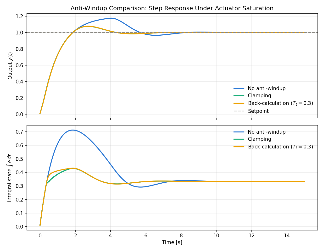
The measured results were:
| Method | Overshoot | Settling time (within 2%) | Peak integral state |
|---|---|---|---|
| No anti-windup | 17.71% | 7.32 s | 0.7127 |
| Clamping | 7.67% | 3.94 s | 0.4301 |
| Back-calculation (\(T_t=0.3\) ) | 7.86% | 3.95 s | 0.4318 |
Without anti-windup, the integral state builds up to around 0.71, and the overshoot worsens to about 17.7% with the settling time nearly doubling to 7.32 seconds. Clamping and back-calculation show almost equivalent improvement (overshoot roughly halved, settling time substantially shortened) — and with \(T_t=0.3\) , back-calculation behaves nearly identically to clamping (the integral-state trajectories in the figure almost overlap).
Discretization Error: Backward, Forward, and Bilinear Transforms
The discrete PID law of Equation (1) approximated the integral with backward difference — accumulating the current sample’s error at each step. We now analyze the frequency-domain error this approximation introduces, comparing it against two other standard discretization methods: forward difference and the bilinear (Tustin) transform.
Three discretization methods
Writing the update rule for the integral state \(I[k] \approx \int_0^{k\Delta t} e(\tau)d\tau\) and its \(z\) -transform for the three standard ways of discretizing the continuous-time integrator \(1/s\) :
Backward Euler reflects the current sample’s error immediately.
\[ I[k] = I[k-1] + \Delta t \, e[k] \quad\Longleftrightarrow\quad \frac{I(z)}{E(z)} = \frac{\Delta t \, z}{z-1} \tag{6} \]Forward Euler reflects only the error up to one sample earlier (the current integral state does not include the current error).
\[ I[k] = I[k-1] + \Delta t \, e[k-1] \quad\Longleftrightarrow\quad \frac{I(z)}{E(z)} = \frac{\Delta t}{z-1} \tag{7} \]The bilinear (Tustin) transform, or trapezoidal rule, averages the current and previous samples’ errors.
\[ I[k] = I[k-1] + \frac{\Delta t}{2}\big(e[k] + e[k-1]\big) \quad\Longleftrightarrow\quad \frac{I(z)}{E(z)} = \frac{\Delta t}{2}\cdot\frac{z+1}{z-1} \tag{8} \]Frequency warping
The bilinear transform corresponds to the algebraic substitution \(s = \dfrac{2}{\Delta t}\cdot\dfrac{z-1}{z+1}\) . Substituting a point on the unit circle, \(z = e^{j\omega\Delta t}\) , gives
\[ \frac{z-1}{z+1} = \frac{e^{j\omega\Delta t}-1}{e^{j\omega\Delta t}+1} = j\tan\!\left(\frac{\omega \Delta t}{2}\right) \]Thus, evaluating the bilinear-discretized integrator at an actual angular frequency \(\omega\) gives a response equivalent to evaluating the continuous-time integrator at the following “warped” angular frequency:
\[ \omega' = \frac{2}{\Delta t}\tan\!\left(\frac{\omega \Delta t}{2}\right) \]While \(\omega \Delta t\) is small (sampling is sufficiently fine), \(\omega' \approx \omega\) , but as it approaches the Nyquist frequency (\(\omega \Delta t \to \pi\) ), \(\tan\) diverges and the frequency response is severely distorted. This is the frequency warping characteristic of the bilinear transform. Backward difference, by contrast, corresponds to the different substitution \(s = \dfrac{z-1}{z\Delta t}\) , under which the imaginary axis \(j\omega\) maps not to the unit circle but to the circle \(|z - 1/2| = 1/2\) — so the distortion of the integrator’s input-output relationship takes a different form than under the bilinear transform.
Verification: comparing stability and tracking performance
For a first-order plant (\(K=1\) , \(T=1\) ) discretized exactly under zero-order hold (ZOH) as \(y[k+1] = a\,y[k] + b\,u[k]\) (with \(a = e^{-\Delta t/T}\) , \(b=K(1-a)\) ), we discretized a PI controller with \(K_P=2.0\) , \(K_I=1.0\) using each of the three methods above, computed the roots of the closed-loop characteristic equation, and used bisection to find the largest sampling period \(\Delta t\) for which both root magnitudes stay below 1 (i.e., the system remains stable).
import numpy as np

K_plant, T_plant = 1.0, 1.0
Kp, Ki = 2.0, 1.0

def poles(dt, method):
    """Closed-loop characteristic-equation roots for an exactly ZOH-discretized
    first-order plant combined with a PI controller discretized by `method`."""
    a = np.exp(-dt / T_plant)
    b = K_plant * (1 - a)
    if method == "backward":
        c1 = -(1 + a) + b * Kp + b * Ki * dt
        c0 = a - b * Kp
    elif method == "forward":
        c1 = -(1 + a) + b * Kp
        c0 = a - b * Kp + b * Ki * dt
    elif method == "tustin":
        c1 = -(1 + a) + b * Kp + b * Ki * dt / 2
        c0 = a - b * Kp + b * Ki * dt / 2
    return np.roots([1.0, c1, c0])

def is_stable(dt, method):
    return np.all(np.abs(poles(dt, method)) < 1.0)

print("Stability boundary (largest dt keeping both poles inside the unit circle):")
for method in ["backward", "forward", "tustin"]:
    lo, hi = 0.01, 5.0
    if is_stable(hi, method):
        print(f"  {method}: stable even at dt={hi}")
        continue
    for _ in range(60):
        mid = (lo + hi) / 2
        lo, hi = (mid, hi) if is_stable(mid, method) else (lo, mid)
    print(f"  {method}: boundary dt ~ {lo:.3f} s")

# Time-domain response near the backward-difference stability boundary (dt=0.8s)
from scipy.integrate import solve_ivp

def simulate(dt, method, t_end=30.0, setpoint=1.0):
    y, integral, prev_error = 0.0, 0.0, 0.0
    t_hist, y_hist = [0.0], [0.0]
    for k in range(int(t_end / dt)):
        error = setpoint - y
        if method == "backward":
            integral += error * dt
            i_term = Ki * integral
        elif method == "forward":
            i_term = Ki * integral
            integral += error * dt
        elif method == "tustin":
            integral += (error + prev_error) / 2 * dt
            i_term = Ki * integral
        u = Kp * error + i_term
        prev_error = error
        sol = solve_ivp(lambda tt, yy: (K_plant * u - yy) / T_plant, [0, dt], [y])
        y = sol.y[0, -1]
        t_hist.append(t_hist[-1] + dt)
        y_hist.append(y)
    return np.array(t_hist), np.array(y_hist)

print("\nTime response at dt=0.8s:")
for method in ["backward", "tustin", "forward"]:
    t_hist, y_hist = simulate(0.8, method)
    overshoot = (np.max(y_hist) - 1.0) * 100
    tol = 0.02
    settle_idx = next((i for i in range(len(y_hist)) if np.all(np.abs(y_hist[i:] - 1.0) < tol)), None)
    settle_t = t_hist[settle_idx] if settle_idx is not None else None
    print(f"  {method:9s}: overshoot={overshoot:.2f}%, settle_t={settle_t}")
Stability boundary (largest dt keeping both poles inside the unit circle):
  backward: boundary dt ~ 0.872 s
  forward: boundary dt ~ 3.000 s
  tustin: boundary dt ~ 1.099 s

Time response at dt=0.8s:
  backward : overshoot=54.18%, settle_t=19.200000000000006
  tustin   : overshoot=32.16%, settle_t=7.199999999999999
  forward  : overshoot=10.13%, settle_t=4.8
| Discretization method | Stability boundary \(\Delta t\) |
|---|---|
| Backward difference | ~0.872 s |
| Bilinear transform | ~1.099 s |
| Forward difference | ~3.0 s or more |
We also simulated the time response at \(\Delta t = 0.8\) s (just below the backward-difference stability boundary):
| Discretization method | Overshoot | Settling time (within 2%) |
|---|---|---|
| Backward difference | 54.18% | 19.2 s |
| Bilinear transform | 32.16% | 7.2 s |
| Forward difference | 10.13% | 4.8 s |
Up to about \(\Delta t \le 0.5\) s, the responses of all three methods are nearly identical (none overshoot at \(\Delta t = 0.5\) s), so as long as sampling is sufficiently fine relative to the plant time constant \(T=1\) , the choice of discretization method does not matter. As \(\Delta t\) becomes coarse relative to \(T\) , however, the differences become apparent, and in this example forward difference turns out to have both the largest stability margin and the best tracking performance. This is because forward difference introduces a one-sample delay into the integral path, which keeps the effective loop gain per sample lower than backward difference or the bilinear transform at coarse \(\Delta t\) . This does not mean forward difference is generally superior, though — this delay normally acts as an undesirable extra dead time. In practice, the standard guidance is to use backward difference or the bilinear transform and choose \(\Delta t\) at roughly a tenth or less of the plant’s dominant time constant (\(\Delta t \lesssim T/10\) ), operating in a regime where the discretization error itself is negligible.
Derivative Kick and Derivative-on-Measurement PID
The problem: output spikes on setpoint changes
The derivative term in Equation (1) is computed from the difference in the error \(e[k] = r[k] - y[k]\) , i.e., \(\dfrac{e[k]-e[k-1]}{\Delta t}\) . Decomposing this into the setpoint’s and the measurement’s respective differences,
\[ \frac{e[k]-e[k-1]}{\Delta t} = \frac{r[k]-r[k-1]}{\Delta t} - \frac{y[k]-y[k-1]}{\Delta t} \]At the instant the setpoint \(r\) changes stepwise (\(r[k] \ne r[k-1]\) ), the first term on the right becomes a finite jump \(\Delta r\) divided by \(\Delta t\) — a very large value for small \(\Delta t\) . This produces an instantaneous, large spike in the control output, known as derivative kick.
The solution: derivative-on-measurement
This problem can be avoided by having the derivative term act only on the measurement \(y\) , not on the error \(e\) :
\[ d[k] = -K_D \frac{y[k]-y[k-1]}{\Delta t} \]The measurement \(y(t)\) is a state variable of the plant, and as long as the plant is a physical system with finite bandwidth, it cannot jump stepwise the way a setpoint can. So under this definition, no matter how abrupt the setpoint change, the derivative term produces no spike. Moreover, during intervals where the setpoint is held constant (\(r[k]=r[k-1]\) ), \(e[k]-e[k-1] = -(y[k]-y[k-1])\) holds, so derivative-on-measurement returns exactly the same value as the ordinary derivative term. In other words, it removes the setpoint-change kick without sacrificing any disturbance-rejection or noise-response characteristics.
Verification
Using a first-order plant (\(K=1\) , \(T=1\) ) with a PID controller at \(K_P=2.0\) , \(K_I=1.0\) , \(K_D=0.5\) , we stepped the setpoint from \(1.0\) to \(2.0\) at \(t=5\) s and compared the control output under the ordinary derivative (derivative-on-error) and derivative-on-measurement.
import numpy as np

class FirstOrderSystem:
    def __init__(self, gain, time_constant, dt):
        self.gain = gain
        self.time_constant = time_constant
        self.dt = dt
        self.y = 0.0
    def update(self, u):
        self.y += self.dt / self.time_constant * (self.gain * u - self.y)
        return self.y

class PIDErrorDerivative:
    """Standard form: the derivative acts on the error e = r - y."""
    def __init__(self, kp, ki, kd, dt):
        self.kp, self.ki, self.kd, self.dt = kp, ki, kd, dt
        self.integral = 0.0
        self.prev_error = None
    def update(self, setpoint, measured):
        error = setpoint - measured
        if self.prev_error is None:
            self.prev_error = error
        self.integral += error * self.dt
        p = self.kp * error
        i = self.ki * self.integral
        d = self.kd * (error - self.prev_error) / self.dt
        self.prev_error = error
        return p + i + d

class PIDMeasurementDerivative:
    """Derivative-on-measurement: the derivative acts on -y only."""
    def __init__(self, kp, ki, kd, dt):
        self.kp, self.ki, self.kd, self.dt = kp, ki, kd, dt
        self.integral = 0.0
        self.prev_measured = None
    def update(self, setpoint, measured):
        error = setpoint - measured
        if self.prev_measured is None:
            self.prev_measured = measured
        self.integral += error * self.dt
        p = self.kp * error
        i = self.ki * self.integral
        d = -self.kd * (measured - self.prev_measured) / self.dt
        self.prev_measured = measured
        return p + i + d

dt = 0.01
t = np.arange(0, 12.0, dt)
setpoint = np.where(t < 5.0, 1.0, 2.0)  # setpoint step at t=5s

for name, cls in [("Derivative-on-error", PIDErrorDerivative),
                   ("Derivative-on-measurement", PIDMeasurementDerivative)]:
    pid = cls(kp=2.0, ki=1.0, kd=0.5, dt=dt)
    plant = FirstOrderSystem(gain=1.0, time_constant=1.0, dt=dt)
    u_hist = []
    for sp in setpoint:
        u = pid.update(sp, plant.y)
        plant.update(u)
        u_hist.append(u)
    u_hist = np.array(u_hist)
    idx_step = np.argmax(t >= 5.0)
    print(f"{name}: u just before step={u_hist[idx_step-1]:.4f}, "
          f"u just after step={u_hist[idx_step]:.4f}, "
          f"jump={u_hist[idx_step]-u_hist[idx_step-1]:.4f}")
Derivative-on-error: u just before step=0.9852, u just after step=52.9953, jump=52.0101
Derivative-on-measurement: u just before step=0.9852, u just after step=2.9953, jump=2.0101
| Form | \(u\) just before the step | \(u\) just after the step | Change |
|---|---|---|---|
| Derivative-on-error (ordinary) | 0.9852 | 52.9953 | +52.010 |
| Derivative-on-measurement | 0.9852 | 2.9953 | +2.010 |
The ordinary derivative term produces a violent kick, jumping the control output to about 53 at the instant of the setpoint step, whereas derivative-on-measurement stays within a mild change of only about 2.01 — essentially just the proportional term’s jump (\(K_P \Delta r = 2.0\) ). Because such a spike on real actuator hardware can cause mechanical shock or saturation, derivative-on-measurement is now close to standard practice in real implementations.
Handling Dead Time and Sensor Noise
Dead time and the limits of PID control
When a plant has dead time \(L\) — due to transport delay, communication latency, or a chemical process’s reaction delay — its transfer function takes the form
\[ G(s) = \frac{K}{1+Ts} e^{-Ls} \]The phase lag from the dead time is \(-\omega L\) [rad], which grows without bound as frequency increases. This phase lag occurs regardless of the controller structure (whether P, PI, or PID), so the larger \(L\) is, the smaller the available phase margin, lowering the maximum gain that keeps the loop stable and preventing the response from being sped up (the fact that all of the Ziegler-Nichols gain formulas were inversely proportional to \(L\) reflects exactly this constraint).
For systems with a large \(L/T\) ratio, this constraint becomes practically unavoidable. A classical remedy is the Smith predictor, proposed by Smith (1957). The basic idea is to embed a mathematical model \(\hat{G}(s)\) of the plant (the part without the dead time) inside the controller, use the model’s delay-free predicted output as the feedback signal, and correct for model error or disturbances using the difference between the actual measurement and the model’s delayed prediction. If the model is accurate, the controller can effectively be tuned as if the system had no dead time, relaxing the stability-limit constraint imposed by \(L\) . Its performance, however, depends strongly on model accuracy, so its benefit is limited for systems with significant modeling error.
Sensor noise and derivative amplification
The derivative term has a frequency-domain gain of \(K_D \cdot j\omega\) , growing in proportion to the angular frequency \(\omega\) . Since measurement noise generally has components across a wide frequency band, a naive derivative (the backward difference of Equation (1)) greatly amplifies it. A widely used countermeasure in practice is the filtered derivative, which adds a first-order low-pass filter to the derivative term.
\[ D(s) = \frac{K_D s}{1 + s/N} = \frac{K_D N s}{s + N} \]\(N\) is called the derivative filter coefficient, and sets the filter’s corner angular frequency (time constant \(\tau_f = 1/N\) ). Its frequency response is
\[ |D(j\omega)| = \frac{K_D N \omega}{\sqrt{\omega^2+N^2}} \]For \(\omega \ll N\) , \(|D(j\omega)| \approx K_D \omega\) , matching the ideal derivative, while for \(\omega \to \infty\) it saturates at \(K_D N\) , so high-frequency noise is no longer amplified without bound. In a discrete implementation, the standard approach (Åström & Hägglund, 1995) is to pass the raw derivative estimate \(d_{raw}[k] = -K_D(y[k]-y[k-1])/\Delta t\) through a first-order lag filter, discretized with backward difference:
\[ d_{filt}[k] = d_{filt}[k-1] + \frac{\Delta t}{\tau_f}\big(d_{raw}[k] - d_{filt}[k-1]\big) \]Verification: the effect of the filtered derivative under sensor noise
For a first-order plant (\(K=1\) , \(T=1\) ) with Gaussian noise of standard deviation 0.01 added to the measurement, we ran PID control at \(K_P=2.0\) , \(K_I=1.0\) , \(K_D=0.5\) under three configurations — no filter, \(N=10\) , and \(N=2\) (a stronger filter) — and compared the control output’s variability and tracking error at steady state (\(t>5\) s).
import numpy as np

class FirstOrderSystem:
    def __init__(self, gain, time_constant, dt):
        self.gain = gain
        self.time_constant = time_constant
        self.dt = dt
        self.y = 0.0
    def update(self, u):
        self.y += self.dt / self.time_constant * (self.gain * u - self.y)
        return self.y

class PIDFilteredDerivative:
    """Derivative-on-measurement with an optional first-order low-pass filter
    of time constant 1/N applied to the raw derivative estimate."""
    def __init__(self, kp, ki, kd, dt, N=None):
        self.kp, self.ki, self.kd, self.dt = kp, ki, kd, dt
        self.N = N
        self.integral = 0.0
        self.prev_measured = None
        self.d_filt = 0.0
    def update(self, setpoint, measured):
        error = setpoint - measured
        if self.prev_measured is None:
            self.prev_measured = measured
        self.integral += error * self.dt
        p = self.kp * error
        i = self.ki * self.integral
        d_raw = -(measured - self.prev_measured) / self.dt
        self.prev_measured = measured
        if self.N is None:
            d_used = d_raw
        else:
            tau_f = 1.0 / self.N
            alpha = min(self.dt / tau_f, 1.0)
            self.d_filt += alpha * (d_raw - self.d_filt)
            d_used = self.d_filt
        return p + i + self.kd * d_used

dt = 0.01
t = np.arange(0, 15.0, dt)
setpoint = np.ones_like(t)
noise_std = 0.01

for label, N in [("No filter", None), ("N=10", 10.0), ("N=2 (stronger filter)", 2.0)]:
    np.random.seed(42)
    pid = PIDFilteredDerivative(kp=2.0, ki=1.0, kd=0.5, dt=dt, N=N)
    plant = FirstOrderSystem(gain=1.0, time_constant=1.0, dt=dt)
    y_hist, u_hist = [], []
    for sp in setpoint:
        noisy_measurement = plant.y + np.random.normal(0, noise_std)
        u = pid.update(sp, noisy_measurement)
        y = plant.update(u)
        y_hist.append(y)
        u_hist.append(u)
    y_hist, u_hist = np.array(y_hist), np.array(u_hist)
    mask = t > 5.0  # steady-state segment
    u_std = np.std(u_hist[mask])
    u_ptp = np.ptp(u_hist[mask])
    tracking_rmse = np.sqrt(np.mean((y_hist[mask] - 1.0) ** 2))
    print(f"{label}: std(u)={u_std:.4f}, ptp(u)={u_ptp:.4f}, tracking_RMSE={tracking_rmse:.5f}")
No filter: std(u)=1.0377, ptp(u)=7.2849, tracking_RMSE=0.01069
N=10: std(u)=0.0717, ptp(u)=0.4361, tracking_RMSE=0.00876
N=2 (stronger filter): std(u)=0.0301, ptp(u)=0.1786, tracking_RMSE=0.00792
| Filter setting | Std. dev. of \(u\) | Peak-to-peak of \(u\) | Tracking RMSE |
|---|---|---|---|
| No filter | 1.0377 | 7.2849 | 0.01069 |
| \(N=10\) | 0.0717 | 0.4361 | 0.00876 |
| \(N=2\) (stronger filter) | 0.0301 | 0.1786 | 0.00792 |
Without filtering, the control output oscillates violently (std. dev. 1.04, peak-to-peak 7.28); with \(N=10\) this is reduced roughly 14.5-fold, to a standard deviation of 0.072. Strengthening the filter further to \(N=2\) smooths the output even more, and the tracking RMSE also improves slightly (a side effect of the filter suppressing the noise itself). Checking the noise-free transient response (settling time), we found essentially no difference — 5.60 s with no filter, 5.55 s at \(N=10\) , and 5.41 s at \(N=2\) — so in this configuration, even a fairly aggressive filter has negligible impact on tracking performance. That said, if the filter time constant \(\tau_f=1/N\) is made too large relative to the plant’s response speed, the resulting phase lag becomes non-negligible and erodes stability margin, so in practice \(N\) is typically searched starting from a few to a few dozen times the reciprocal of the plant’s dominant time constant.
Ziegler-Nichols Tuning Method
The Ziegler-Nichols method is a classical approach for empirically determining PID gains from the plant’s step response characteristics. Here we introduce the step response method (open-loop method).
Step Response Method
A step input is applied to the plant, and the following three parameters are read from the response curve:
- \(K\) : Process gain (steady-state value / input value)
- \(L\) : Dead time (delay before the response begins)
- \(T\) : Time constant (time from the inflection point tangent to reaching the steady-state value)
Based on these parameters, PID gains are calculated using the following table.
| Controller | \(K_P\) | \(T_I\) | \(T_D\) |
|---|---|---|---|
| P | \(\frac{T}{KL}\) | - | - |
| PI | \(\frac{0.9T}{KL}\) | \(\frac{L}{0.3}\) | - |
| PID | \(\frac{1.2T}{KL}\) | \(2L\) | \(0.5L\) |
Here, \(T_I\) is the integral time and \(T_D\) is the derivative time, with the relationships \(K_I = K_P / T_I\) and \(K_D = K_P \cdot T_D\) .
The Ziegler-Nichols method tends to produce oscillatory responses as its starting point, so the resulting gains often lead to significant overshoot. In practice, these values are used as initial settings and then fine-tuned manually.
Disturbance Rejection Simulation
In real control systems, disturbances (unexpected external inputs) affect control performance. Here we add a step disturbance midway through the simulation and compare the disturbance rejection of P control and PID control.
import numpy as np
import matplotlib.pyplot as plt

dt = 0.01
t_end = 20.0
t = np.arange(0, t_end, dt)
setpoint = np.ones_like(t)

# Disturbance: step of magnitude 0.5 at t=10s
disturbance = np.zeros_like(t)
disturbance[t >= 10.0] = 0.5

plant_params = {'gain': 1.0, 'time_constant': 1.0, 'dt': dt}

configs = [
    ('P control (Kp=2.0)', {'kp': 2.0, 'ki': 0.0, 'kd': 0.0}),
    ('PID control (Kp=2.0, Ki=1.0, Kd=0.5)', {'kp': 2.0, 'ki': 1.0, 'kd': 0.5}),
]

fig, axes = plt.subplots(2, 1, figsize=(10, 8), sharex=True)

for label, params in configs:
    pid = PIDController(**params, dt=dt)
    plant = FirstOrderSystem(**plant_params)
    y_hist = []
    u_hist = []

    for i, sp in enumerate(setpoint):
        u = pid.update(sp, plant.y)
        # Add disturbance to plant input
        y = plant.update(u + disturbance[i])
        y_hist.append(y)
        u_hist.append(u)

    axes[0].plot(t, y_hist, label=label)
    axes[1].plot(t, u_hist, label=label)

axes[0].axhline(y=1.0, color='k', linestyle='--', alpha=0.5, label='Setpoint')
axes[0].axvline(x=10.0, color='r', linestyle=':', alpha=0.5, label='Disturbance onset')
axes[0].set_ylabel('Output y(t)')
axes[0].set_title('Disturbance Rejection Comparison')
axes[0].legend()
axes[0].grid(True, alpha=0.3)

axes[1].set_ylabel('Control input u(t)')
axes[1].set_xlabel('Time [s]')
axes[1].legend()
axes[1].grid(True, alpha=0.3)

plt.tight_layout()
plt.show()
The simulation results show the following:
- P control: It provides some disturbance suppression, but a steady-state error due to the disturbance remains.
- PID control: Thanks to the integral term, the output eventually returns to the setpoint even after the disturbance is applied. The derivative term also improves the initial response to the disturbance.
Recent Trends: Auto-Tuning and Choosing Between PID and MPC
Classical tuning methods such as Ziegler-Nichols remain a widely used starting point in practice, but since 2023 research has become increasingly active in automating gain search as an optimization problem.
Gain search via reinforcement learning: Sönmez et al. (arXiv:2502.04552, 2025) propose online tuning of quadrotor attitude-control PID gains using DDPG (Deep Deterministic Policy Gradient), adjusting gains sequentially during flight, and report tracking accuracy that exceeds hand-tuned baselines both in simulation and in actual flight tests. The Gaussian-process surrogate-model-based search covered in Bayesian Optimization: Fundamentals and Python Implementation is also being applied to PID tuning. Fujimoto et al. (2023, Asian Journal of Control) validate controller tuning via Bayesian optimization and its acceleration, both conceptually and experimentally, and report that encoding prior knowledge of the plant model into the acquisition function’s prior mean can substantially reduce the number of trials required.
Choosing between PID and MPC: Recent work has also clarified when to prefer PID over more advanced control methods such as MPC or ML-based controllers. Sarhadi (arXiv:2503.14379, 2025) reports that under nominal conditions (an idealized setting free of saturation, disturbance, noise, and model error), PID and MPC perform comparably, but under realistic operating conditions with saturation, disturbance, sensor noise, and model uncertainty, constrained MPC substantially outperforms PID — while PID with anti-windup maintains reasonable performance. This is consistent with the anti-windup effect we derived in this article, and offers a practical takeaway: there is no need to bring in MPC’s added complexity where PID suffices, but in settings where saturation and constraints dominate performance, the quality of the anti-windup implementation itself is what determines the performance gap between PID and MPC. Because this field is moving quickly, we recommend consulting the primary sources for specific performance figures and methodological details.
Summary
In this article, we implemented a PID controller in Python and verified its behavior through simulation with a first-order system. By comparing P, PI, and PID step responses, we experimentally confirmed the role and effect of each component. We further derived four implementation issues that are unavoidable in practice — anti-windup (back-calculation, clamping, and conditional integration), discretization error (backward difference, forward difference, and the bilinear transform), derivative kick and derivative-on-measurement PID, and handling dead time and sensor noise (the filtered derivative) — and confirmed each one’s effect through numerical experiments.
PID control is simple in structure yet achieves high control performance when tuned and implemented with these practical considerations in mind. However, for systems with strong nonlinearity, multiple inputs and outputs, or systems where handling constraints is fundamentally important, more advanced control methods become necessary.
Related Articles
- Bode Plot: Reading and Creating Frequency Response Diagrams with Python Implementation - Defines gain margin and phase margin and numerically verifies a case where GM is sufficient but PM is not — the foundation for evaluating stability limits during PID gain tuning.
- Nyquist Plot, Root Locus, and Stability Margins in Python - How to quantify the stability limit when raising PID gains, using gain/phase margins and the root locus — the follow-up that backs this article’s gain tuning with a stability analysis.
- Fundamentals of PID Control and the Role of Each Component - Explains the mathematical definitions of P, PI, and PID control and the characteristics of each component.
- Mathematics of MPPI (Model Predictive Path Integral) - Introduces model predictive control based on Monte Carlo sampling as an advanced control method beyond PID.
- Kalman Filter: Theory and Python Implementation - Explains state estimation methods used in combination with feedback control.
- Fundamentals of Filtering Methods in Signal Processing - Provides an overview of filtering methods used for state estimation in control systems.
- Matplotlib Practical Tips: Creating Publication-Quality Plots - Introduces settings for creating higher-quality plots of simulation results.
- Moving Average Filters Compared: SMA, WMA, and EMA in Python - Because the PID derivative term is sensitive to noise, moving averages (SMA/WMA/EMA) are commonly used to smooth sensor inputs before they are fed into the controller.
- Complementary Filter: Theory and Python Implementation - A lightweight attitude estimator widely used to produce the feedback signal consumed by PID controllers.
References
- Astrom, K. J., & Murray, R. M. (2021). Feedback Systems: An Introduction for Scientists and Engineers (2nd ed.). Princeton University Press.
- Ziegler, J. G., & Nichols, N. B. (1942). “Optimum settings for automatic controllers”. Transactions of the ASME, 64(11), 759-768.
- Åström, K. J., & Hägglund, T. (1995). PID Controllers: Theory, Design, and Tuning (2nd ed.). Instrument Society of America.
- Smith, O. J. M. (1957). “Closer control of loops with dead time”. Chemical Engineering Progress, 53(5), 217-219.
- Fujimoto, Y., Sato, H., & Nagahara, M. (2023). “Controller tuning with Bayesian optimization and its acceleration: Concept and experimental validation”. Asian Journal of Control, 25(6).
- Sönmez, S., Montecchio, L., Martini, S., Rutherford, M. J., Rizzo, A., Stefanovic, M., & Valavanis, K. P. (2025). “Reinforcement Learning Based Prediction of PID Controller Gains for Quadrotor UAVs”. arXiv:2502.04552.
- Sarhadi, P. (2025). “On the Standard Performance Criteria for Applied Control Design: PID, MPC or Machine Learning Controller?”. arXiv:2503.14379.