Introduction
Time series forecasting is essential across domains including demand planning, financial analysis, and weather prediction. ARIMA (AutoRegressive Integrated Moving Average) is a classical yet powerful time series forecasting method.
This article derives the mathematics of AR, MA, ARIMA, and SARIMA from the roots of characteristic polynomials on the unit circle — rather than stating them by fiat — and walks through the Box-Jenkins method (identification → estimation → diagnostic checking) end to end in Python. The theoretical background of exact Kalman-filter maximum likelihood estimation is covered in depth in https://yuhi-sa.github.io/en/posts/20260715_arima_state_space_kalman/1/, and the detailed derivation of order identification via the PACF is covered in https://yuhi-sa.github.io/en/posts/20260710_pacf_ar_identification/1/. This article instead focuses on running the practical Box-Jenkins workflow (stationarity testing → order identification → conditional MLE → residual diagnostics → forecasting) through a single worked example from start to finish.
AR (AutoRegressive) Model
The AR(\(p\) ) model expresses the current value using the past \(p\) values:
\[X_t = c + \sum_{i=1}^{p} \phi_i X_{t-i} + \varepsilon_t \tag{1}\]where \(\phi_i\) are autoregressive coefficients and \(\varepsilon_t \sim \mathcal{N}(0, \sigma^2)\) is white noise.
Deriving the stationarity condition
Take the AR(1) model \(X_t = \phi X_{t-1} + \varepsilon_t\) as a concrete case to see why the magnitude of the coefficient determines stationarity. Substituting backward \(k\) times gives
\[X_t = \phi^k X_{t-k} + \sum_{j=0}^{k-1} \phi^j \varepsilon_{t-j} \tag{2}\]As \(k \to \infty\) , if \(|\phi| < 1\) then \(\phi^k X_{t-k} \to 0\) (mean-square convergence), leaving
\[X_t = \sum_{j=0}^{\infty} \phi^j \varepsilon_{t-j} \tag{3}\]— a causal MA(∞) representation built purely from past shocks with finite variance. The variance is the sum of a geometric series,
\[ \mathrm{Var}(X_t) = \sigma^2 \sum_{j=0}^{\infty} \phi^{2j} = \frac{\sigma^2}{1 - \phi^2} < \infty \]which is finite and well defined. Conversely, if \(|\phi| > 1\) the term \(\phi^k X_{t-k}\) in equation (2) diverges, and at \(|\phi| = 1\) (a unit root, i.e. a random walk) the variance grows without bound over time — neither case gives a process with a time-invariant, finite variance.
The characteristic equation of AR(1) is \(1 - \phi z = 0\) , with root \(z = 1/\phi\) . Therefore
\[|\phi| < 1 \iff |z| = \left|\frac{1}{\phi}\right| > 1\]— stationarity is equivalent to the root lying outside the unit circle. This correspondence extends to the general AR(\(p\) ) case. Writing the characteristic equation as
\[1 - \phi_1 z - \phi_2 z^2 - \cdots - \phi_p z^p = 0\]with roots \(z_1, \ldots, z_p\) , a partial-fraction expansion shows that \(1/\phi(z)\) can be written as a power series \(\sum_j \psi_j z^j\) in \(z\) , whose radius of convergence is exactly \(\min_i |z_i|\) . For the coefficients \(\{\psi_j\}\) to be absolutely summable (\(\sum_j |\psi_j| < \infty\) , i.e. for a causal MA(∞) representation to exist), the radius of convergence must exceed \(1\) :
\[\min_i |z_i| > 1\]All roots must lie outside the unit circle — this is the necessary and sufficient condition for AR(\(p\) ) to admit a stationary MA(∞) representation.
Checking this against the AR(2) process used in the numerical experiment below (\(\phi_1=0.5, \phi_2=-0.3\) ), the characteristic equation \(1 - 0.5z + 0.3z^2 = 0\) has roots \(z = 0.8333 \pm 1.6245i\) with modulus \(|z| = 1.8257 > 1\) , confirming stationarity (we reproduce this numerically in the Python code below).
MA (Moving Average) Model
The MA(\(q\) ) model is a linear combination of past \(q\) noise terms:
\[X_t = \mu + \varepsilon_t + \sum_{j=1}^{q} \theta_j \varepsilon_{t-j} \tag{4}\]Since this is a finite sum of stationary terms, the MA model is always stationary regardless of the \(\theta_j\) values.
Deriving invertibility
Stationarity is automatic, but a separate condition — invertibility — is needed to identify parameters uniquely from data. Consider MA(1): \(X_t = \varepsilon_t + \theta \varepsilon_{t-1}\) . Using the backshift operator \(B\) (\(B\varepsilon_t = \varepsilon_{t-1}\) ), we can write \(X_t = (1+\theta B)\varepsilon_t\) , and formally expanding the inverse operator gives
\[ \varepsilon_t = (1+\theta B)^{-1} X_t = \sum_{j=0}^{\infty} (-\theta)^j X_{t-j} \]an AR(∞) representation. This series converges (i.e. the current shock \(\varepsilon_t\) can be recovered from past observations alone) exactly when \(|\theta| < 1\) . The characteristic equation \(1 + \theta z = 0\) has root \(z = -1/\theta\) , so this is the same unit-circle condition as AR stationarity, just applied to the MA polynomial.
The need for invertibility comes down to parameter non-uniqueness. The theoretical ACF of MA(1) is
\[\rho_1 = \frac{\theta}{1+\theta^2}\]which is unchanged under \(\theta \to 1/\theta\) (for example, \(\theta=2\) and \(\theta=0.5\) produce identical autocorrelation structure). The ACF alone cannot distinguish \(\theta\) from \(1/\theta\) , so by convention we pick the root satisfying \(|\theta|<1\) to fix a unique representation. For a general MA(\(q\) ), invertibility requires all roots of \(\theta(z) = 1 + \theta_1 z + \cdots + \theta_q z^q\) to lie outside the unit circle.
ARMA Model
Combining AR and MA gives ARMA(\(p, q\) ):
\[X_t = c + \sum_{i=1}^{p} \phi_i X_{t-i} + \varepsilon_t + \sum_{j=1}^{q} \theta_j \varepsilon_{t-j} \tag{5}\]Stationarity is judged from the roots of the AR characteristic polynomial and invertibility from the roots of the MA polynomial, independently of each other. Both must hold for the parameters to be uniquely identifiable in a stationary process.
ARIMA Model
For non-stationary series, apply \(d\) differences to achieve stationarity, then fit ARMA. This is ARIMA(\(p, d, q\) ):
\[\Delta^d X_t = c + \sum_{i=1}^{p} \phi_i \Delta^d X_{t-i} + \varepsilon_t + \sum_{j=1}^{q} \theta_j \varepsilon_{t-j} \tag{6}\]where \(\Delta X_t = X_t - X_{t-1}\) is the first difference.
- \(p\) : autoregressive order
- \(d\) : differencing order (typically 0, 1, or 2)
- \(q\) : moving average order
Parameter Estimation via Conditional Maximum Likelihood
The Box-Jenkins method is a three-stage, iterative framework: identification → estimation → diagnostic checking. Here we derive the estimation stage’s core tool, conditional sum-of-squares (CSS) maximum likelihood.
For an AR(\(p\) ) model with \(\varepsilon_t \sim \mathcal{N}(0, \sigma^2)\) , equation (1) implies the Markov property
\[ X_t \mid X_{t-1}, \ldots, X_{t-p} \sim \mathcal{N}\!\left(c + \sum_{i=1}^{p} \phi_i X_{t-i},\ \sigma^2\right) \]Conditioning on the first \(p\) observations \(X_1, \ldots, X_p\) , the joint density factors as a product of these conditional distributions:
\[ f(x_{p+1}, \ldots, x_N \mid x_1, \ldots, x_p) = \prod_{t=p+1}^{N} f(x_t \mid x_{t-1}, \ldots, x_{t-p}) \]Taking logarithms, the conditional log-likelihood is
\[ \ell_c(\phi, \sigma^2) = -\frac{N-p}{2}\ln(2\pi\sigma^2) - \frac{1}{2\sigma^2}\sum_{t=p+1}^{N}\left(x_t - c - \sum_{i=1}^{p}\phi_i x_{t-i}\right)^{2} \tag{7} \]Maximizing equation (7) over \(\phi_i\) for fixed \(\sigma^2\) is equivalent to minimizing the residual sum of squares in the second term — that is, exactly ordinary least squares (OLS) regressing \(x_t\) on \(x_{t-1}, \ldots, x_{t-p}\) . This is why the method is called “conditional sum of squares” (CSS). Substituting \(\hat{\phi}\) and solving \(\partial \ell_c/\partial \sigma^2 = 0\) gives the MLE
\[\hat{\sigma}^2 = \frac{1}{N-p}\sum_{t=p+1}^{N}\left(x_t - \hat{c} - \sum_i \hat{\phi}_i x_{t-i}\right)^2\]the residual sum of squares divided by the effective sample size. The same idea extends to general ARMA models, but since MA terms involve unobserved \(\varepsilon_{t-j}\) , one typically initializes \(\varepsilon_0 = \varepsilon_{-1} = \cdots = 0\) or backcasts before assembling the conditional likelihood.
CSS is computationally simple, but it is an approximation that discards the marginal-distribution information carried by the first \(p\)
observations. An alternative incorporates the stationary distribution of \(X_1, \ldots, X_p\)
as the initial condition and computes the exact (approximation-free) Gaussian log-likelihood for the entire observed sequence via the Kalman filter’s prediction-error decomposition — this is what statsmodels’ ARIMA class uses internally by default. The derivation of this exact likelihood, and a numerical comparison against CSS, is covered in depth in https://yuhi-sa.github.io/en/posts/20260715_arima_state_space_kalman/1/. Later in this article’s Python implementation, we compare a hand-rolled CSS estimator against statsmodels’ exact MLE numerically.
Parameter Selection (the identification step)
ACF and PACF
| Pattern | ACF | PACF | Model |
|---|---|---|---|
| AR(\(p\) ) | Gradual decay | Sharp cutoff at lag \(p\) | Use PACF for p |
| MA(\(q\) ) | Sharp cutoff at lag \(q\) | Gradual decay | Use ACF for q |
| ARMA(\(p,q\) ) | Gradual decay | Gradual decay | Use AIC/BIC |
Why the PACF cuts off for an AR process (it is the correlation left after removing the linear effect of intermediate lags), and the concrete calculation via the Yule-Walker equations and the Levinson-Durbin recursion, are developed in full — with both derivations and numerical experiments — in https://yuhi-sa.github.io/en/posts/20260710_pacf_ar_identification/1/. Here we take this identification table as given and move directly to plotting and reading off orders in Python.
Information Criteria
Use AIC or BIC to select the optimal \((p, d, q)\) combination:
\[\text{AIC} = -2\ln(L) + 2k \tag{8}\]where \(L\) is maximum likelihood and \(k\) is the number of parameters.
Python Implementation: From Stationarity Testing to Model Estimation
Data generation and the ADF test
We generate data from a true AR(2) process (\(\phi_1=0.5, \phi_2=-0.3\) ) plus a linear trend, and check stationarity with the Augmented Dickey-Fuller (ADF) test.
import numpy as np
import pandas as pd
from statsmodels.tsa.arima.model import ARIMA
from statsmodels.tsa.stattools import adfuller

# --- Generate data (AR(2) process + trend) ---
np.random.seed(42)
n = 300
noise = np.random.normal(0, 1, n)
data = np.zeros(n)
for t in range(2, n):
    data[t] = 0.5 * data[t-1] - 0.3 * data[t-2] + noise[t]
data += np.linspace(0, 10, n)  # add a trend

ts = pd.Series(data, index=pd.date_range('2024-01-01', periods=n, freq='D'))

# --- Verify the AR(2) characteristic roots numerically ---
roots = np.roots([-(-0.3), -(0.5), 1])  # 1 - 0.5z + 0.3z^2 = 0
print("characteristic roots:", roots, "moduli:", np.abs(roots))

# --- Stationarity test (ADF test) ---
result = adfuller(ts)
print(f"ADF statistic: {result[0]:.4f}, p-value: {result[1]:.4f}")
print("critical values:", result[4])

ts_diff = ts.diff().dropna()
result_diff = adfuller(ts_diff)
print(f"After 1st diff - ADF: {result_diff[0]:.4f}, p-value: {result_diff[1]:.4f}")
Output:
characteristic roots: [0.83333333+1.62446572j 0.83333333-1.62446572j] moduli: [1.82574186 1.82574186]
ADF statistic: -0.1789, p-value: 0.9410
critical values: {'1%': -3.4532, '5%': -2.8716, '10%': -2.5721}
After 1st diff - ADF: -7.6752, p-value: 0.0000
critical values (diff): {'1%': -3.4538, '5%': -2.8718, '10%': -2.5723}
The root modulus \(1.8257\) matches the theoretical value derived above, confirming the AR(2) component is stationary. But because the full series includes a linear trend, the ADF statistic (\(-0.1789\) , above every critical value, \(p=0.9410\) ) fails to reject the unit-root null — the series appears non-stationary. After first-differencing, the ADF statistic (\(-7.6752\) , well below the 1% critical value of \(-3.4538\) , \(p \approx 0\) ) clearly indicates stationarity, numerically confirming \(d=1\) is appropriate.
Identifying orders from ACF/PACF plots
import matplotlib.pyplot as plt
from statsmodels.graphics.tsaplots import plot_acf, plot_pacf

fig, axes = plt.subplots(1, 2, figsize=(12, 4))
plot_acf(ts_diff, ax=axes[0], lags=20, title='ACF (1st Difference)')
plot_pacf(ts_diff, ax=axes[1], lags=20, method='ywm', title='PACF (1st Difference)')
plt.tight_layout()
plt.show()
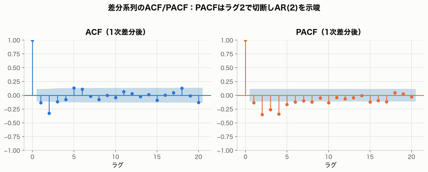
The PACF cuts off at lag 2, suggesting an AR(2) component per the identification table (why AR structure survives in the differenced series is explained in the “overdifferencing” section below).
Numerical comparison: conditional MLE (CSS) vs. exact MLE
We implement the conditional least-squares estimator derived above by hand and compare it to statsmodels’ exact (Kalman-filter-based) estimation.
train = ts[:250]
test = ts[250:]

# --- Manual conditional MLE (CSS) ---
y = train.diff().dropna().values
X = np.column_stack([y[1:-1], y[0:-2]])  # lag 1, lag 2
yt = y[2:]
beta = np.linalg.lstsq(X, yt, rcond=None)[0]
resid_css = yt - X @ beta
sigma2_css = np.sum(resid_css**2) / len(resid_css)
print("[CSS] phi1, phi2:", beta, "sigma2:", sigma2_css)

# --- statsmodels exact MLE (Kalman-filter-based) ---
fitted = ARIMA(train, order=(2, 1, 0)).fit()
print("[exact MLE] phi1, phi2:", fitted.arparams, "sigma2:", fitted.params.iloc[-1])
print(fitted.summary())
Output:
[CSS] phi1, phi2: [-0.14256314 -0.3405605 ] sigma2: 1.3407 (n=247)
[exact MLE] phi1, phi2: [-0.14198861 -0.33822858] sigma2: 1.3316 (llf=-389.10, N=249)

                 coef    std err          z      P>|z|
ar.L1         -0.1420      0.067     -2.125      0.034
ar.L2         -0.3382      0.064     -5.307      0.000
sigma2         1.3316      0.120     11.059      0.000
AIC: 784.19   BIC: 794.74
CSS (\(\hat{\phi}_1=-0.1426, \hat{\phi}_2=-0.3406\) ) and statsmodels’ exact MLE (\(\hat{\phi}_1=-0.1420, \hat{\phi}_2=-0.3382\) ) agree to 2-3 decimal places. The small discrepancy comes from CSS conditioning away — and thus losing — the first two points (effective \(N=247\) ), whereas the exact MLE uses the stationary distribution as an initial condition and exploits all \(N=249\) points. The Kalman filter’s prediction-error decomposition, derived in https://yuhi-sa.github.io/en/posts/20260715_arima_state_space_kalman/1/, is precisely the mechanism that closes this gap.
Residual Diagnostics and a Model-Selection Pitfall: Overdifferencing
As the third Box-Jenkins stage, “diagnostic checking,” we run the Ljung-Box test to see whether residuals behave like white noise.
from statsmodels.stats.diagnostic import acorr_ljungbox

lb = acorr_ljungbox(fitted.resid, lags=[10, 20], return_df=True)
print(lb)
Output:
      lb_stat     lb_pvalue
10  48.436410  5.165530e-07
20  60.495144  5.968126e-06
Both lags are rejected at \(p < 0.001\) — significant autocorrelation remains in the residuals. Even though the ADF test supported stationarity after first-differencing, and the PACF showed a cutoff at lag 2, ARIMA(2,1,0) turns out to be misspecified.
The culprit is overdifferencing. This article’s data-generating process is “a stationary AR(2) plus a deterministic linear trend” — it has no stochastic unit root. Yet applying a first difference (\(d=1\) ) to an already-stationary AR(2) process artificially introduces a non-invertible MA component (for AR(1) as an illustration: \(x_t - x_{t-1} = \phi(x_{t-1}-x_{t-2}) + (\varepsilon_t - \varepsilon_{t-1})\) , and the right-hand term \(\varepsilon_t - \varepsilon_{t-1}\) generates an MA(1) component). Trying to model this artificial MA structure with ARIMA(2,1,0) — MA order 0 — leaves residual structure behind.
We fix this two ways and compare AIC, residual diagnostics, and forecast error.
# Fix 1: add an MA term to absorb the artificial MA component
m211 = ARIMA(train, order=(2, 1, 1)).fit()
lb211 = acorr_ljungbox(m211.resid, lags=[10, 20], return_df=True)

# Fix 2: skip differencing, model the deterministic trend explicitly (matches the true DGP)
m200t = ARIMA(train, order=(2, 0, 0), trend='t').fit()
lb200t = acorr_ljungbox(m200t.resid, lags=[10, 20], return_df=True)

for name, m, lb in [("ARIMA(2,1,0)", fitted, lb), ("ARIMA(2,1,1)", m211, lb211), ("ARIMA(2,0,0)+trend", m200t, lb200t)]:
    fc = m.forecast(steps=len(test))
    rmse = np.sqrt(np.mean((test.values - fc.values)**2))
    mae = np.mean(np.abs(test.values - fc.values))
    print(f"{name}: AIC={m.aic:.2f}, LB(10) p={lb['lb_pvalue'].iloc[0]:.3f}, RMSE={rmse:.4f}, MAE={mae:.4f}")
Output:
| Model | AIC | Ljung-Box(10) p-value | RMSE | MAE |
|---|---|---|---|---|
| ARIMA(2,1,0) (misspecified) | 784.19 | 5.2×10⁻⁷ (rejected) | 1.2494 | 0.9762 |
| ARIMA(2,1,1) | 725.46 | 0.211 (white noise) | 1.5652 | 1.2807 |
| ARIMA(2,0,0)+trend (true specification) | 698.94 | 0.562 (white noise) | 1.1196 | 0.8848 |
The model matching the true data-generating process — ARIMA(2,0,0)+trend — is best on AIC, residual diagnostics, and forecast error alike. Yet if you looked at AIC alone, ARIMA(2,1,0) is worse than ARIMA(2,1,1), whereas on point-forecast RMSE alone, ARIMA(2,1,0) (1.2494) looks better than ARIMA(2,1,1) (1.5652). That’s a coincidence specific to this test window; once residuals fail the white-noise check, the reliability of the forecast intervals is no longer guaranteed. Never judge a model by AIC or point-forecast RMSE alone — always pair it with residual diagnostics (the Ljung-Box test): that is the essence of the Box-Jenkins method.
For reference, a naive “carry the last value forward” forecast gives RMSE \(= 1.4017\) and MAE \(= 1.1301\) . ARIMA(2,1,0) beats this naive baseline, but still falls short of the true specification, ARIMA(2,0,0)+trend.
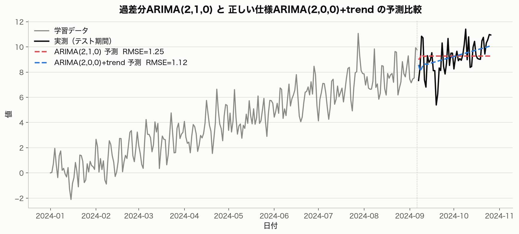
The overdifferenced ARIMA(2,1,0) (red dashed) fails to track the trend’s rise during the test period and stays nearly flat, while the correctly specified ARIMA(2,0,0)+trend (blue dashed) tracks the trend closely — a difference that is visually obvious as well.
SARIMA (Seasonal ARIMA)
For seasonal data, use SARIMA(\(p, d, q\) )(\(P, D, Q\) )\(_s\) :
\[\Phi_P(B^s) \phi_p(B) \Delta^d \Delta_s^D X_t = \Theta_Q(B^s) \theta_q(B) \varepsilon_t \tag{9}\]where \(s\) is the seasonal period (12 for monthly data) and \(B\) is the backshift operator (\(BX_t = X_{t-1}\) ).
Numerical experiment: how much worse is it to ignore seasonality?
We generate 180 months of data from a true SARIMA(1,1,1)(1,1,1,12) process (via SARIMAX.simulate, with \(\phi=0.5, \theta=-0.4, \Phi=0.3, \Theta=-0.5\)
), run the ADF test after seasonal differencing, fit SARIMAX, and compare forecasts against a non-seasonal ARIMA(1,1,1) that ignores the seasonal structure.
from statsmodels.tsa.statespace.sarimax import SARIMAX
from statsmodels.tsa.arima.model import ARIMA
from statsmodels.tsa.stattools import adfuller
from statsmodels.stats.diagnostic import acorr_ljungbox

n = 180
dummy = pd.Series(np.zeros(n), index=pd.date_range('2010-01-01', periods=n, freq='MS'))
mod = SARIMAX(dummy, order=(1, 1, 1), seasonal_order=(1, 1, 1, 12), trend='n')
true_params = [0.5, -0.4, 0.3, -0.5, 1.0]  # ar, ma, ar.S, ma.S, sigma2
sim = mod.simulate(true_params, n, initial_state=np.zeros(mod.k_states),
                    random_state=9) + 50  # random_state ensures reproducibility
ts_s = pd.Series(sim.values, index=dummy.index)
train_s, test_s = ts_s[:150], ts_s[150:]

# ADF test after seasonal differencing
res_sd = adfuller(ts_s.diff(12).dropna())
print(f"ADF after seasonal diff: {res_sd[0]:.4f}, p-value: {res_sd[1]:.4f}")

# SARIMA model
sarima_fit = SARIMAX(train_s, order=(1, 1, 1), seasonal_order=(1, 1, 1, 12)).fit(disp=False)
lb_s = acorr_ljungbox(sarima_fit.resid.iloc[13:], lags=[12, 24], return_df=True)
fc_s = sarima_fit.get_forecast(steps=len(test_s)).predicted_mean
rmse_s = np.sqrt(np.mean((test_s.values - fc_s.values)**2))
mae_s = np.mean(np.abs(test_s.values - fc_s.values))

# Non-seasonal ARIMA that ignores seasonality
nonseason_fit = ARIMA(train_s, order=(1, 1, 1)).fit()
fc_ns = nonseason_fit.forecast(steps=len(test_s))
rmse_ns = np.sqrt(np.mean((test_s.values - fc_ns.values)**2))
mae_ns = np.mean(np.abs(test_s.values - fc_ns.values))

print(f"SARIMA: AIC={sarima_fit.aic:.2f}, RMSE={rmse_s:.3f}, MAE={mae_s:.3f}")
print(f"Non-seasonal ARIMA: AIC={nonseason_fit.aic:.2f}, RMSE={rmse_ns:.3f}, MAE={mae_ns:.3f}")
print(lb_s)
Output:
ADF after seasonal diff: -3.4639, p-value: 0.0090

SARIMA(1,1,1)(1,1,1,12): AIC=384.24, RMSE=3.872, MAE=3.595
      lb_stat  lb_pvalue
12   8.024676   0.783199
24  14.797854   0.926534

Non-seasonal ARIMA(1,1,1): AIC=685.03, RMSE=7.720, MAE=6.421
The ADF statistic after seasonal differencing (\(-3.4639\) , \(p=0.0090\) ) confirms stationarity, and the SARIMA residuals pass the Ljung-Box white-noise test (\(p=0.783, 0.927\) ). The non-seasonal ARIMA(1,1,1), which ignores seasonality, is much worse: AIC \(685.03\) versus SARIMA’s \(384.24\) , and RMSE/MAE deteriorate by roughly 2.0×/1.8× (RMSE: \(3.872 \to 7.720\) ; MAE: \(3.595 \to 6.421\) ). This is direct numerical evidence for the value of modeling the seasonal period explicitly.
Note that SARIMAX.simulate maintains its own internal random state, so setting np.random.seed() globally alone does not make the results reproducible. Passing an explicit integer to the random_state argument, as in the code above, is what makes the generated series reproducible run to run — another easy-to-miss pitfall when working with seasonal models.
Automated Model Selection (auto_arima) and Its Limits
pmdarima’s auto_arima can search for optimal parameters automatically, but by nature of the search algorithm, it does not always find the best model.
import pmdarima as pm

# Default: stepwise search (Hyndman-Khandakar algorithm)
auto_stepwise = pm.auto_arima(train, seasonal=False, stepwise=True, suppress_warnings=True)
print("stepwise selection:", auto_stepwise.order, "AIC:", auto_stepwise.aic())

# Exhaustive search (stepwise=False)
auto_full = pm.auto_arima(train, seasonal=False, stepwise=False, suppress_warnings=True,
                           max_p=5, max_q=5, max_d=2, n_jobs=-1)
print("full-search selection:", auto_full.order, "AIC:", auto_full.aic())
Output:
stepwise selection: (0, 1, 0) AIC: 813.02
full-search selection: (5, 1, 0) AIC: 732.96
The default stepwise search picks ARIMA(0,1,0) (AIC \(813.02\)
) — essentially “do nothing” — which is worse than the manually compared ARIMA(2,1,0) (AIC \(784.19\)
) from earlier. Switching to stepwise=False for an exhaustive search improves things slightly to ARIMA(5,1,0) (AIC \(732.96\)
), but this still falls short of the true specification, ARIMA(2,0,0)+trend (AIC \(698.94\)
). This exposes two independent issues.
- Stepwise search can get stuck in a local optimum:
stepwise=Truedoes not search the entire candidate space, and as we see here, it can land far from the optimum. - The search space itself does not contain the true model:
auto_arima(seasonal=False)only searches the differencing order \(d\) and AR/MA orders — it never includes a deterministic trend term as a candidate. When the trend is deterministic rather than a stochastic unit root, as here, no amount of increasing the AR/MA order can reach the true specification; the only recourse is to over-parameterize (\(p=5\) ) as an approximation.
Automated tools are ultimately heuristic searches within a given candidate space — domain knowledge about the data-generating process (whether the trend is deterministic or stochastic, whether seasonality is present, etc.) is still required to design that search space.
Practical Notes
- Watch for overdifferencing: relying solely on the ADF test and the PACF identification table can lead you to difference a stationary process that has a deterministic trend. Always confirm residual whiteness with the Ljung-Box test after differencing.
- Watch the invertibility boundary: when an estimated MA coefficient lands near \(\pm 1\)
(the non-invertible boundary), standard errors can blow up dramatically (in a preliminary experiment for this article, an overdifferenced case with both seasonal and non-seasonal differencing applied together showed
ma.L1’s standard error inflate by several hundredfold). That is a sign to reconsider the order or the number of differences. - AIC and point-forecast RMSE are different metrics: in this article’s numerical experiments, a model rejected by residual diagnostics still looked better on RMSE for a particular test window. Check AIC, residual diagnostics, and forecast error together, as a set.
- Automated tools are not a silver bullet:
auto_arima’s stepwise search can get stuck in local optima, and designing the search space (whether to include a trend term, whether to search seasonality) remains the user’s responsibility.
Recent Research
The practical trade-off between the classical Box-Jenkins method (ARIMA) and machine learning approaches continues to be actively studied. Tjøstheim (2025), Selected Topics in Time Series Forecasting: Statistical Models vs. Machine Learning (Entropy 27(3), 279, DOI: 10.3390/e27030279), reviews results across the Makridakis forecasting competitions (M1-M6) and shows that classical linear parametric models such as ARIMA and exponential smoothing remain competitive with machine learning on low-frequency (“well-behaved,” low spectral-entropy) series such as monthly data, while machine learning gains a clear edge in domains dominated by nonlinearity and variance clustering, such as volatility forecasting and high-frequency financial data. The Theta method — an extension of exponential smoothing — won M3, and a hybrid of exponential smoothing and deep learning won M4, underscoring that the recent trend is “combine classical statistics with machine learning” rather than “statistics versus machine learning.” This reinforces the point that ARIMA is not a universal model but one tool to be chosen based on the properties of the data at hand — its linearity and entropy.
Python Implementation Summary
# The final model combining the above, close to the true specification
final_model = ARIMA(train, order=(2, 0, 0), trend='t').fit()
print(final_model.summary())
forecast = final_model.get_forecast(steps=len(test))
mean_forecast = forecast.predicted_mean
conf_int = forecast.conf_int()
Related Articles
- ARMA/ARIMA in State-Space Form: Kalman-Filter Maximum Likelihood Estimation - Derives the Kalman-filter-based exact likelihood that statsmodels’ ARIMA estimation uses internally, and numerically checks it against this article’s conditional MLE (CSS).
- PACF and AR Model Order Identification - A deep dive into this article’s order-selection step: the Yule-Walker equations, the Levinson-Durbin recursion, and identifying the AR order \(p\) from the PACF.
- GARCH(1,1) in Python - A complementary model for the variance clustering (volatility clustering) that this article’s model cannot capture.
- Machine Learning for Time-Series Prediction, Classification, and Anomaly Detection Hub - Compares ARIMA with k-means / GMM / RF / GBDT / LSTM / Kalman / IsolationForest and gives a selection guideline.
- Time-Series Forecasting with LSTM - LSTM handles nonlinear long-range dependencies that ARIMA’s linear formulation cannot.
- Digital Signal Processing and Machine Learning Roadmap - Meta roadmap that places ARIMA within the five-hub learning path.
- Time-Series Anomaly Detection: From Statistical Methods to Kalman Filter in Python - Using ARIMA prediction deviations for anomaly detection.
- Moving Average Filters Compared: SMA, WMA, and EMA in Python - Provides intuitive understanding of MA models.
- Kalman Filter: Theory and Python Implementation - State-space model-based time series estimation; useful comparison with ARIMA.
- Matplotlib Practical Tips: Creating Publication-Quality Figures - Tips for high-quality time series visualization.
- Frequency Characteristics of the EMA Filter - EMA is a time series smoothing method related to the MA component of ARIMA.
- Bayesian Linear Regression: From Least Squares to Bayesian Estimation - Bayesian approaches to time series regression.
References
- Box, G. E. P., Jenkins, G. M., Reinsel, G. C., & Ljung, G. M. (2015). Time Series Analysis: Forecasting and Control (5th ed.). Wiley.
- Hyndman, R. J., & Athanasopoulos, G. (2021). Forecasting: Principles and Practice (3rd ed.).
- Tjøstheim, D. (2025). “Selected Topics in Time Series Forecasting: Statistical Models vs. Machine Learning.” Entropy, 27(3), 279. DOI: 10.3390/e27030279
- statsmodels ARIMA documentation