Introduction
The Butterworth filter is an IIR filter with a maximally flat magnitude response in the passband. Published by Stephen Butterworth in 1930, it features a smooth frequency response with no ripple and is one of the most widely used filter designs in signal processing.
This article covers the mathematical foundations of the Butterworth filter through practical design and implementation with SciPy.
Magnitude Response
Magnitude Squared Function
The magnitude squared function of an \(N\) -th order Butterworth lowpass filter is:
\[|H(j\Omega)|^2 = \frac{1}{1 + \left(\frac{\Omega}{\Omega_c}\right)^{2N}} \tag{1}\]where \(\Omega_c\) is the cutoff angular frequency (-3dB point) and \(N\) is the filter order.
Maximally Flat Property
Taylor expansion of equation \((1)\) around \(\Omega = 0\) shows that the first \(2N-1\) derivatives of \(|H(j\Omega)|^2\) are all zero. This is why it is called “maximally flat.”
Behavior by Frequency
- \(\Omega = 0\) : \(|H| = 1\) (perfect passthrough)
- \(\Omega = \Omega_c\) : \(|H| = 1/\sqrt{2} \approx -3\,\text{dB}\)
- \(\Omega \gg \Omega_c\) : \(|H| \approx (\Omega_c/\Omega)^N\) (roll-off rate: \(-20N\) dB/decade)
Pole Locations
Butterworth filter poles are equally spaced on a circle of radius \(\Omega_c\) (the Butterworth circle) in the s-plane. The \(k\) -th pole of an \(N\) -th order filter is:
\[s_k = \Omega_c \exp\left(j\frac{\pi(2k + N - 1)}{2N}\right), \quad k = 1, 2, \ldots, N \tag{2}\]Only poles in the left half-plane (negative real part) are used for a stable filter.
Design Procedure
1. Determine Filter Order
Compute the required order from passband/stopband specifications:
\[N \geq \frac{\log(\varepsilon_s^2/\varepsilon_p^2)}{2\log(\Omega_s/\Omega_p)} \tag{3}\]2. Analog Prototype Design
Design a normalized Butterworth filter with \(\Omega_c = 1\) .
3. Digital Conversion
Convert the analog filter to digital using the bilinear transform:
\[s = \frac{2}{T}\frac{1 - z^{-1}}{1 + z^{-1}} \tag{4}\]Pre-warping compensates for the frequency axis distortion:
\[\Omega_a = \frac{2}{T}\tan\left(\frac{\omega_d T}{2}\right) \tag{5}\]Numerical Verification: Skipping Pre-Warping Overestimates the Order
Equation \((3)\) uses the ratio of analog angular frequencies
\[ \Omega_s/\Omega_p \]but a common mistake in digital filter design is plugging in the raw frequency ratio directly. Let’s verify with a concrete specification how much the required order changes with and without pre-warping.
Specification: sampling frequency \(f_s = 1000\) Hz, passband edge \(f_p = 100\) Hz, stopband edge \(f_{st} = 300\) Hz, passband ripple \(R_p = 1\) dB, stopband attenuation \(R_s = 40\) dB.
import numpy as np
from scipy import signal

fs = 1000                 # Sampling frequency [Hz]
fp, fst = 100, 300         # Passband / stopband edges [Hz]
rp, rs = 1, 40             # Passband ripple [dB] / stopband attenuation [dB]

eps_p = np.sqrt(10**(rp / 10) - 1)
eps_s = np.sqrt(10**(rs / 10) - 1)

# (a) Without pre-warping: plug the raw frequency ratio into eq. (3) (incorrect)
N_naive = np.log10(eps_s**2 / eps_p**2) / (2 * np.log10(fst / fp))

# (b) With pre-warping: correct the angular frequencies with tan first (correct)
T = 1 / fs
Wp = (2 / T) * np.tan(2 * np.pi * fp * T / 2)
Wst = (2 / T) * np.tan(2 * np.pi * fst * T / 2)
N_prewarp = np.log10(eps_s**2 / eps_p**2) / (2 * np.log10(Wst / Wp))

# (c) Cross-check against scipy.signal.buttord's automatic design
N_buttord, wn = signal.buttord(fp / (fs / 2), fst / (fs / 2), rp, rs)

print(f"Without pre-warping: N = {N_naive:.3f} -> order used {int(np.ceil(N_naive))}")
print(f"With pre-warping:    N = {N_prewarp:.3f} -> order used {int(np.ceil(N_prewarp))}")
print(f"buttord:             N = {N_buttord} (Wn = {wn:.4f})")
Output:
Without pre-warping: N = 4.807 -> order used 5
With pre-warping:    N = 3.658 -> order used 4
buttord:             N = 4 (Wn = 0.2338)
Skipping pre-warping treats the raw frequency ratio
\[ f_{st}/f_p = 3.0 \]directly, overestimating the required order at 5th order. Pre-warping with \(\tan\) , on the other hand, stretches the stopband edge’s angular frequency more strongly because it sits close to the Nyquist frequency (\(500\) Hz), expanding the effective frequency ratio to
\[ W_{st}/W_p = 2752.76 / 649.84 = 4.24 \]Using this expanded ratio in equation \((3)\)
gives \(N=3.658\)
, which rounds up to 4th order — exactly matching scipy.signal.buttord. Verifying the 4th-order filter against the specification confirms \(-1.00\)
dB at \(f_p=100\)
Hz (exactly meeting \(R_p=1\)
dB) and \(-44.29\)
dB at \(f_{st}=300\)
Hz (a \(4.29\)
dB margin over the required \(R_s=40\)
dB).
Caveat: scipy.signal.buttord performs this pre-warping internally, so in practice you rarely need to compute equation \((3)\)
by hand. However, if you estimate the order manually or in a spreadsheet, forgetting this correction leads to one extra order than necessary (i.e. unnecessary computational cost and numerical-error risk). The effect grows more pronounced the closer the stopband edge is to the Nyquist frequency — that is, the higher the cutoff frequency relative to the sampling rate.
Python Implementation
Filter Design and Frequency Response with SciPy
import numpy as np
import matplotlib.pyplot as plt
from scipy import signal

# --- Filter design ---
fs = 1000           # Sampling frequency [Hz]
fc = 100            # Cutoff frequency [Hz]
orders = [2, 4, 8]  # Filter orders

fig, axes = plt.subplots(2, 1, figsize=(10, 8))

for N in orders:
    sos = signal.butter(N, fc, fs=fs, output='sos')
    w, h = signal.sosfreqz(sos, worN=4096, fs=fs)

    axes[0].plot(w, 20 * np.log10(np.abs(h) + 1e-12), label=f'N={N}')
    axes[1].plot(w, np.degrees(np.unwrap(np.angle(h))), label=f'N={N}')

axes[0].set_xlabel('Frequency [Hz]')
axes[0].set_ylabel('Magnitude [dB]')
axes[0].set_title('Butterworth Filter - Magnitude Response')
axes[0].set_xlim(0, 500)
axes[0].set_ylim(-80, 5)
axes[0].axvline(fc, color='gray', linestyle='--', alpha=0.5)
axes[0].axhline(-3, color='gray', linestyle=':', alpha=0.5, label='-3 dB')
axes[0].legend()
axes[0].grid(True, alpha=0.3)

axes[1].set_xlabel('Frequency [Hz]')
axes[1].set_ylabel('Phase [degrees]')
axes[1].set_title('Butterworth Filter - Phase Response')
axes[1].set_xlim(0, 500)
axes[1].legend()
axes[1].grid(True, alpha=0.3)

plt.tight_layout()
plt.show()
Numerical Verification of Order-Dependent Gain and Roll-Off
Let’s numerically verify the properties “-3dB at the cutoff frequency” and “roll-off of \(-20N\)
dB/decade” using scipy.signal. We design filters for \(f_c = 100\)
Hz with \(N \in \{2, 4, 6, 8\}\)
and compute the gain at 2x, 10x, and 100x the cutoff frequency.
import numpy as np
from scipy import signal

fs = 100_000   # Use a high sampling rate to observe high frequencies
fc = 100       # Cutoff frequency [Hz]
orders = [2, 4, 6, 8]

print(f"{'N':<4}{'gain@fc[dB]':>14}{'gain@2fc[dB]':>15}{'gain@10fc[dB]':>16}{'gain@100fc[dB]':>17}")
for N in orders:
    sos = signal.butter(N, fc, fs=fs, output='sos')
    freqs = np.array([fc, 2 * fc, 10 * fc, 100 * fc])
    _, h = signal.sosfreqz(sos, worN=freqs, fs=fs)
    gdb = 20 * np.log10(np.abs(h))
    print(f"{N:<4}{gdb[0]:>14.4f}{gdb[1]:>15.4f}{gdb[2]:>16.4f}{gdb[3]:>17.4f}")
Output:
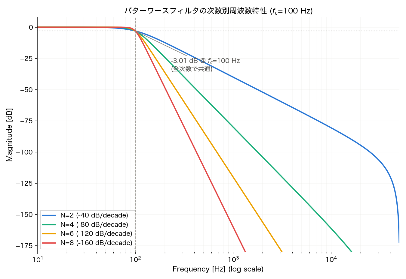
N      gain@fc[dB]   gain@2fc[dB]  gain@10fc[dB]  gain@100fc[dB]
2          -3.0103       -12.3047       -40.0061        -80.5850
4          -3.0103       -24.0997       -80.0113       -161.1700
6          -3.0103       -36.1252      -120.0170       -241.7550
8          -3.0103       -48.1656      -160.0226       -322.3400
The attenuation at \(f_c\) is exactly \(-3.0103\) dB regardless of order (from equation \((1)\) , \(|H(j\Omega_c)|^2 = 1/2\) independent of \(N\) ). Overlaying the frequency responses by order makes the difference in roll-off slope visually clear.
Next, we compute the measured roll-off from the gain change over one decade (\(10f_c\) to \(100f_c\) ) and compare it against the theoretical \(-20N\) dB/decade.
import numpy as np
from scipy import signal

fs = 100_000
fc = 100
orders = [2, 4, 6, 8]

theoretical = [-20 * N for N in orders]
measured = []
for N in orders:
    sos = signal.butter(N, fc, fs=fs, output='sos')
    freqs = np.array([10 * fc, 100 * fc])
    _, h = signal.sosfreqz(sos, worN=freqs, fs=fs)
    gdb = 20 * np.log10(np.abs(h))
    slope = (gdb[1] - gdb[0]) / (np.log10(100 * fc) - np.log10(10 * fc))
    measured.append(slope)

for N, th, ms in zip(orders, theoretical, measured):
    print(f"N={N}: theoretical {th} dB/decade, measured {ms:.3f} dB/decade, diff {ms - th:+.3f} dB")
Output:
N=2: theoretical -40 dB/decade, measured -40.579 dB/decade, diff -0.579 dB
N=4: theoretical -80 dB/decade, measured -81.159 dB/decade, diff -1.159 dB
N=6: theoretical -120 dB/decade, measured -121.738 dB/decade, diff -1.738 dB
N=8: theoretical -160 dB/decade, measured -162.317 dB/decade, diff -2.317 dB
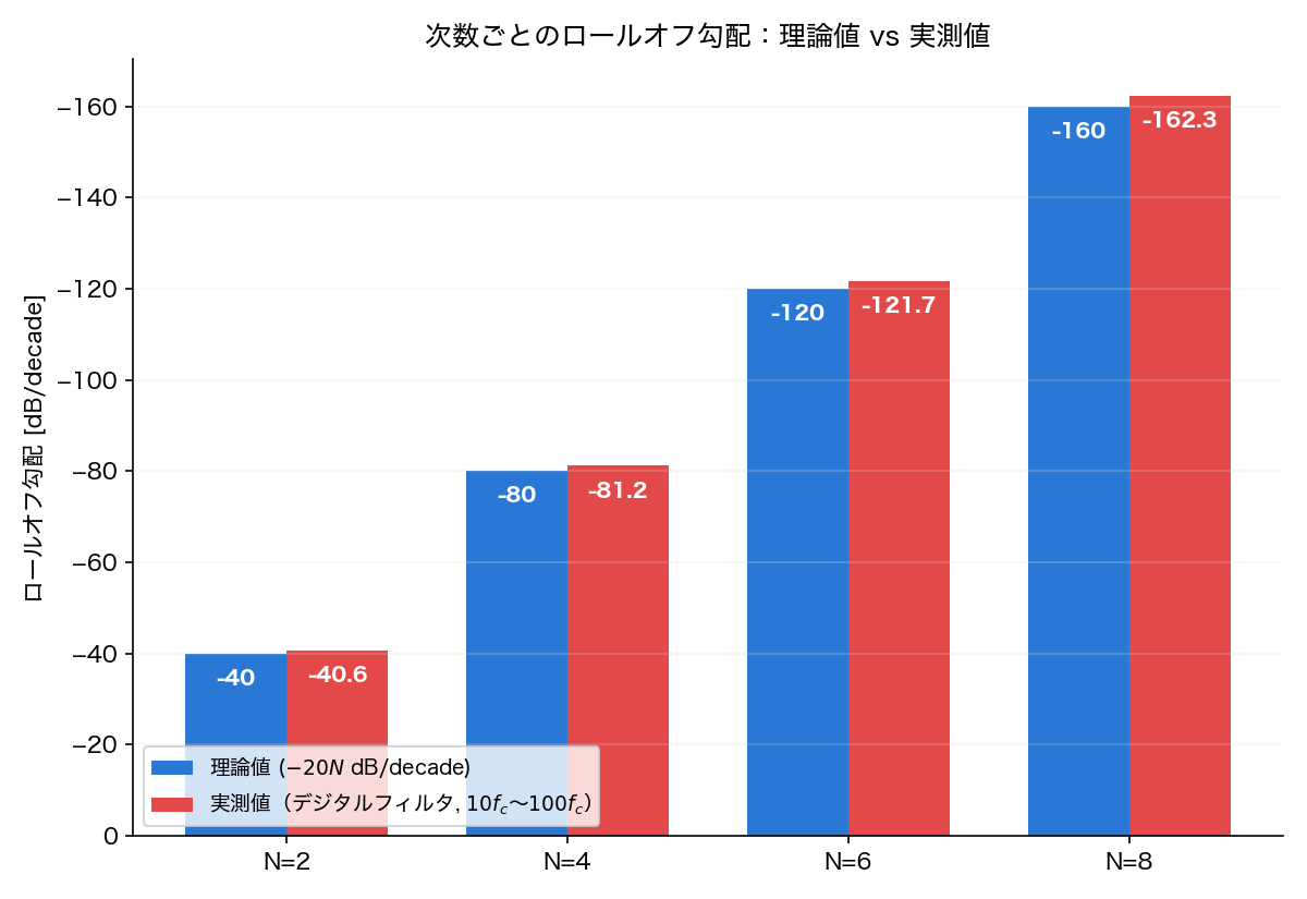
Edge case: the deviation from the theoretical value grows with order. This is because the analog prototype follows exactly \(-20N\)
dB/decade, whereas the bilinear-transformed digital filter compresses the high-frequency axis logarithmically (the warping effect). Indeed, evaluating the same filter as an analog design with signal.butter(..., analog=True) gives slopes of exactly \(-40.000, -80.000, -120.000, -160.000\)
dB/decade for \(N=2,4,6,8\)
over \(10f_c\)
to \(100f_c\)
— matching the theoretical values exactly. In other words, the deviation observed here is not an error in Butterworth theory but an inherent nonlinear frequency-axis distortion of digital IIR filters near the Nyquist frequency — something to watch for when designing high-order filters or filters with a cutoff frequency relatively high compared to the sampling rate.
Noise Removal Application
import numpy as np
import matplotlib.pyplot as plt
from scipy import signal

# --- Generate signal ---
fs = 1000
t = np.arange(0, 1, 1/fs)
clean = np.sin(2 * np.pi * 10 * t) + 0.5 * np.sin(2 * np.pi * 30 * t)
noisy = clean + 0.8 * np.random.randn(len(t))

# --- Design and apply Butterworth filter ---
sos = signal.butter(4, 50, fs=fs, output='sos')
filtered_causal = signal.sosfilt(sos, noisy)       # Causal filter
filtered_zero = signal.sosfiltfilt(sos, noisy)      # Zero-phase filter

# --- Plot ---
fig, axes = plt.subplots(3, 1, figsize=(10, 8), sharex=True)

axes[0].plot(t, noisy, alpha=0.5, label='Noisy')
axes[0].plot(t, clean, 'k', linewidth=1.5, label='Original')
axes[0].set_title('Input Signal')
axes[0].legend()
axes[0].grid(True, alpha=0.3)

axes[1].plot(t, filtered_causal, label='sosfilt (causal)')
axes[1].plot(t, clean, 'k', linewidth=1.5, label='Original')
axes[1].set_title('Causal Filtering (sosfilt)')
axes[1].legend()
axes[1].grid(True, alpha=0.3)

axes[2].plot(t, filtered_zero, label='sosfiltfilt (zero-phase)')
axes[2].plot(t, clean, 'k', linewidth=1.5, label='Original')
axes[2].set_title('Zero-Phase Filtering (sosfiltfilt)')
axes[2].set_xlabel('Time [s]')
axes[2].legend()
axes[2].grid(True, alpha=0.3)

plt.tight_layout()
plt.show()
sosfilt is a causal filter (with phase delay), while sosfiltfilt achieves zero-phase by filtering forward and backward, but cannot be used for real-time processing.
Comparison with Other IIR Filters
| Filter | Passband | Stopband | Transition Band | Phase |
|---|---|---|---|---|
| Butterworth | Maximally flat | Monotonic | Wide | Relatively smooth |
| Chebyshev Type I | Equiripple | Monotonic | Narrow | Steep changes |
| Chebyshev Type II | Monotonic | Equiripple | Narrow | Relatively smooth |
| Elliptic (Cauer) | Equiripple | Equiripple | Narrowest | Steepest |
For the same order, elliptic filters have the sharpest transition band but introduce passband ripple. Butterworth is optimal when ripple is unacceptable. For a quantitative comparison of order and group delay across filter types (including a side-by-side minimum-order comparison via buttord, cheb1ord, cheb2ord, and ellipord), see
Elliptic (Cauer) Filter: Theory and Python Implementation
— this article focuses solely on the Butterworth filter’s own design principles.
Recent Research
Although the Butterworth filter is a classical design from 1930, research on order-determination algorithms and implementation forms continues today. Dey, Roy & Sarkar (2026) applied a novel hybrid metaheuristic optimization algorithm — the Chaotic Quasi-Oppositional Bald Eagle Search (CQOBES), which combines chaotic maps with quasi-oppositional learning — to the design of fractional-order Butterworth filters, a generalization of the conventional integer-order design. They showed the approach minimizes the error to the target response not only for lowpass but also for highpass and bandpass fractional-order Butterworth filters (Circuits, Systems, and Signal Processing, Springer, 2026). Because fractional-order filters allow finer control of the transition characteristic between passband and stopband than integer orders do, they offer a practical advantage in cases where a conventional Butterworth design forces a binary choice of whether to bump the order up by one.
Related Articles
- Low-Pass Filter Design and Comparison - Comparison of various lowpass filters including Butterworth.
- FIR vs IIR Filters: Characteristics, Design, and Python Implementation - Compares Butterworth (IIR) and FIR filter characteristics.
- Wiener Filter: Optimal Linear Filtering Theory and Python Implementation - Contrasts Wiener’s automatic band design with Butterworth’s manual cutoff.
- Notch Filter Design and Python Implementation - IIR filter application for specific frequency removal.
- Fast Fourier Transform (FFT): Theory and Python Implementation - FFT details for analyzing filter frequency characteristics.
- Frequency Characteristics of the EMA Filter - Frequency characteristics of EMA, a first-order IIR filter.
- Moving Average Filters Compared: SMA, WMA, and EMA in Python - Moving average filters as representative FIR filters.
- Fundamentals of Filtering Methods in Signal Processing - Systematic overview of various filters.
- Savitzky-Golay Filter: Theory and Python Implementation - An FIR polynomial fitting filter, contrasting with Butterworth’s IIR approach to smoothing.
- Adaptive Filters (LMS/RLS): Theory and Python Implementation - Unlike Butterworth’s fixed design, adaptive filters automatically adjust parameters based on the input signal.
- Chebyshev Filter Design: Theory and Python Implementation - Equiripple IIR filter that achieves a sharper transition band than Butterworth at the same order.
- Bessel Filter: Theory and Python Implementation - IIR filter that maximizes flat group delay; gentler roll-off than Butterworth but better phase response.
- Elliptic (Cauer) Filter: Theory and Python Implementation - Allows ripple in both passband and stopband to achieve the steepest transition for a given order.
- Bandpass Filter Design and Python Implementation - Derive the bandpass version by frequency-transforming the Butterworth prototype.
- Highpass Filter Design and Python Implementation - Derive the highpass version from the Butterworth LPF prototype to remove low-frequency drift.
- Bode Plot: Theory and Python Implementation - Compare Butterworth’s maximally flat passband and \(-20N\) dB/dec roll-off against other filters on a unified Bode plot view.
- Filter Design Selection Guide: 3 axes and characteristic comparison — Use this hub to position the Butterworth filter against alternatives during selection.
- Z-Transform and Discrete-Time System Theory - The theoretical foundation for discretizing Butterworth designs (bilinear transform) and analyzing the resulting transfer function’s pole-zero placement and stability.
References
- Butterworth, S. (1930). “On the theory of filter amplifiers”. Wireless Engineer, 7(6), 536-541.
- Oppenheim, A. V., & Schafer, R. W. (2009). Discrete-Time Signal Processing (3rd ed.). Prentice Hall.
- Dey, S., Roy, P. K., & Sarkar, A. (2026). “Accurate Design of Digital Fractional-Order Butterworth Filters Using a Novel Chaotic Quasi-Oppositional Bald Eagle Search Algorithm”. Circuits, Systems, and Signal Processing. https://link.springer.com/article/10.1007/s00034-026-03623-1
- SciPy scipy.signal.butter documentation