Introduction
Ensemble learning combines multiple weak learners to achieve higher generalization performance than any single model. Most top solutions in Kaggle competitions employ ensemble methods.
This article systematically covers decision trees as the building block, bagging (Random Forest), and boosting (GBDT).
Decision Trees
CART Algorithm
For classification, recursively find splits minimizing Gini impurity:
\[\text{Gini}(t) = 1 - \sum_{k=1}^{K} p_k^2 \tag{1}\]where \(p_k\) is the proportion of class \(k\) in node \(t\) .
For regression, minimize mean squared error:
\[\text{MSE}(t) = \frac{1}{|t|} \sum_{i \in t} (y_i - \bar{y}_t)^2 \tag{2}\]What Impurity Really Means: Deriving Gini and Entropy
Why minimize “impurity” at all? An impurity function \(\varphi(p_1,\dots,p_K)\) over a node \(t\) needs three properties: (i) it attains its minimum \(0\) at a pure node (some \(p_k=1\) ), (ii) it attains its maximum at the uniform distribution \(p_k=1/K\) , and (iii) it is concave in \(p_k\) . Gini impurity (Eq. 1) and entropy are both canonical examples satisfying these. Entropy, borrowed from information theory, is defined as:
\[ H(t) = -\sum_{k=1}^{K} p_k \log p_k \tag{3} \]The split criterion is maximizing information gain. When a candidate split \(s\) divides node \(t\) into children \(t_L, t_R\) with proportions \(w_L = n_L/n_t\) and \(w_R = n_R/n_t\) , CART greedily picks the split that maximizes the information gain:
\[ \Delta I(s, t) = \varphi(t) - \left[w_L \varphi(t_L) + w_R \varphi(t_R)\right] \tag{4} \]The key fact is that \(\Delta I(s,t) \ge 0\) always holds. Since the count of class \(k\) in \(t\) is the sum of the counts in \(t_L\) and \(t_R\) , the class proportions of \(t\) are a convex combination of the children’s proportions: \(p_k(t) = w_L p_k(t_L) + w_R p_k(t_R)\) . Because \(\varphi\) is concave, Jensen’s inequality gives
\[ \varphi(t) = \varphi\big(w_L\, p(t_L) + w_R\, p(t_R)\big) \ge w_L \varphi(t_L) + w_R \varphi(t_R) \]which is exactly \(\Delta I(s,t)\ge 0\) . In other words, as long as the impurity function is concave, no split can ever make training impurity worse. This is precisely why a decision tree can drive training error arbitrarily low simply by splitting deeper — a property we verify numerically below.
The relationship between Gini and entropy. These are not two independent measures — they are the same quantity at different orders of approximation. From \(\ln x \le x-1\) (equality at \(x=1\) ) we get \(-\ln p_k \ge 1-p_k\) ; multiplying both sides by \(p_k \ge 0\) and summing over \(k\) :
\[ H(t) = \sum_k p_k \ln\frac{1}{p_k} \;\ge\; \sum_k p_k(1-p_k) = 1 - \sum_k p_k^2 = \text{Gini}(t) \]so entropy is always at least as large as Gini impurity. The gap shrinks as each \(p_k\)
approaches 1 (near-pure nodes), because the Taylor expansion \(\ln(1/p_k) = (1-p_k) + \frac{(1-p_k)^2}{2} + \cdots\)
has a first-order term that matches Gini’s summand \(1-p_k\)
exactly. Gini impurity is thus entropy’s first-order (linear) approximation, with entropy exceeding it by the second-order term \((1-p_k)^2/2>0\)
. It is no coincidence that criterion='gini' and 'entropy' tend to produce similar trees in practice — this approximation relationship is why.
Deriving the MSE Split Criterion for Regression Trees
The same “concave function + Jensen’s inequality” structure becomes a fully closed-form variance decomposition for regression trees. Let \(\bar y_L, \bar y_R\) be the child means, \(n=n_L+n_R\) , and \(\bar y = (n_L\bar y_L+n_R\bar y_R)/n\) the overall mean. The sum-of-squares identity
\[ \sum_{i \in t}(y_i - \bar y)^2 = \sum_{i \in t_L}(y_i - \bar y_L)^2 + \sum_{i \in t_R}(y_i - \bar y_R)^2 + \frac{n_L n_R}{n}(\bar y_L - \bar y_R)^2 \]holds (expand the left side by adding and subtracting \(\bar y_L\) or \(\bar y_R\) inside each square; the cross terms vanish because \(\sum_{i\in t_L}(y_i-\bar y_L)=0\) , etc.). Dividing both sides by \(n\) gives the MSE decomposition:
\[ \text{MSE}(t) = w_L\,\text{MSE}(t_L) + w_R\,\text{MSE}(t_R) + w_L w_R (\bar y_L - \bar y_R)^2 \tag{5} \](with \(w_L=n_L/n,\ w_R=n_R/n\) ). The information gain under the MSE criterion is therefore an exact closed form:
\[ \Delta \text{MSE}(s, t) = \text{MSE}(t) - \left[w_L\,\text{MSE}(t_L) + w_R\,\text{MSE}(t_R)\right] = w_L w_R (\bar y_L - \bar y_R)^2 \tag{6} \]which is proportional to the squared difference between the two child means. Whereas Gini’s information gain was only guaranteed to be non-negative via Jensen’s inequality, MSE’s reduction can be written as an exact identity (equality, not just an inequality).
Strengths and Weaknesses
| Strengths | Weaknesses |
|---|---|
| Interpretable | Prone to overfitting |
| No preprocessing needed | Axis-aligned boundaries |
| Handles nonlinearity | High variance (unstable) |
Experiment: Depth Control and Overfitting
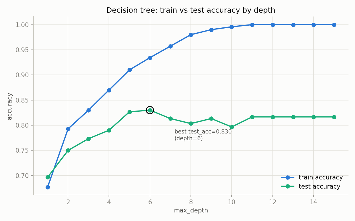
We showed above that a decision tree’s impurity can only decrease as it splits deeper. But how do training and validation accuracy actually diverge as a tree grows deeper? Using the same 1,000-sample, 20-feature make_classification data (700 train / 300 validation, random_state=42, identical to this article’s Python implementation), we trained DecisionTreeClassifier with max_depth swept from 1 to 15 and recorded training and validation accuracy at each depth.
depths = list(range(1, 16))
train_accs, test_accs = [], []
for d in depths:
    clf = DecisionTreeClassifier(max_depth=d, random_state=42)
    clf.fit(X_train, y_train)
    train_accs.append(accuracy_score(y_train, clf.predict(X_train)))
    test_accs.append(accuracy_score(y_test, clf.predict(X_test)))
The results (excerpt):
max_depth | Train acc. | Val. acc. | Gap (overfit) |
|---|---|---|---|
| 1 | 0.677 | 0.697 | -0.020 |
| 3 | 0.830 | 0.773 | 0.057 |
| 5 | 0.910 | 0.827 | 0.083 |
| 6 | 0.934 | 0.830 | 0.104 |
| 8 | 0.980 | 0.803 | 0.177 |
| 10 | 0.996 | 0.797 | 0.199 |
| 15 (actual depth saturates at 11) | 1.000 | 0.817 | 0.183 |
Validation accuracy peaks at 0.830 for max_depth=6; beyond that, training accuracy pins at 1.0 while validation accuracy actually declines to around 0.80 (bottoming out at 0.797 for max_depth=10). The train/validation gap widens roughly monotonically with depth. At max_depth=1, validation accuracy is slightly higher than training accuracy — statistical noise from the small 300-sample validation set rather than a real effect. This result bridges the earlier theorem that impurity can only decrease with splitting (Eq. 4) and the next section’s argument that test error, governed by the bias-variance decomposition, does not necessarily decrease without bound.
The figure below shows this:
Bagging
The Bias-Variance Decomposition
To understand why bagging works, we first need to derive the decomposition of expected squared error. Let the true model be \(y = f(\mathbf{x}) + \varepsilon\) (\(\mathbb{E}[\varepsilon]=0\) , \(\text{Var}(\varepsilon)=\sigma^2\) , \(\varepsilon\) independent of the estimator), and let \(\hat f_D(\mathbf x)\) be an estimator trained on training set \(D\) . We evaluate the expected squared error at a new point \((\mathbf x, y)\) , taking expectation over both \(D\) and \(\varepsilon\) . Writing \(\bar f(\mathbf x) := \mathbb{E}_D[\hat f_D(\mathbf x)]\) (the estimator’s average across training sets),
\[ \mathbb{E}_{D,\varepsilon}\big[(y - \hat f_D(\mathbf x))^2\big] = \mathbb{E}\Big[\big((f(\mathbf x) - \bar f(\mathbf x)) + (\bar f(\mathbf x) - \hat f_D(\mathbf x)) + \varepsilon\big)^2\Big] \]Expanding the right side gives three squared terms and three cross terms, and every cross term vanishes: \((f-\bar f)\) is a constant depending only on \(\mathbf x\) , so \(\mathbb{E}_D[\bar f(\mathbf x) - \hat f_D(\mathbf x)] = \bar f(\mathbf x)-\bar f(\mathbf x)=0\) kills the cross term between the first two pieces, and \(\varepsilon\) ’s independence from both \(\hat f_D\) and \(f\) with zero mean kills every cross term involving \(\varepsilon\) . Only the three squared terms survive:
$$ \mathbb{E}{D,\varepsilon}\big[(y - \hat f_D(\mathbf x))^2\big] = \underbrace{(f(\mathbf x)-\bar f(\mathbf x))^2}{\text{Bias}^2}
- \underbrace{\mathbb{E}D\big[(\bar f(\mathbf x) - \hat f_D(\mathbf x))^2\big]}{\text{Variance}}
- \sigma^2 \tag{7} $$
This is the bias-variance decomposition. Bagging targets only the Variance term — it does not, in principle, touch the Bias or the irreducible noise \(\sigma^2\) .
Principle
Bootstrap Aggregating (bagging) trains multiple decision trees on bootstrap samples independently, then averages (regression) or votes (classification):
\[\hat{f}_{\text{bag}}(\mathbf{x}) = \frac{1}{B} \sum_{b=1}^{B} \hat{f}_b(\mathbf{x}) \tag{8}\]This reduces variance:
\[\text{Var}\left(\frac{1}{B}\sum_b f_b\right) = \frac{\sigma^2}{B} \quad (\text{if independent}) \tag{9}\]Bootstrap Correlation and the Limit of Variance Reduction
Eq. (9) assumes the \(B\) trees are perfectly independent — unrealistic, since every tree is trained on a bootstrap sample drawn from the same \(n\) points, which induces positive correlation between trees. Let \(\sigma_f^2 := \text{Var}(\hat f_b)\) be each tree’s variance and \(\rho\) the pairwise correlation between any two trees. The variance of the averaged predictor \(\hat f_{\text{bag}} = \frac1B\sum_b \hat f_b\) in general is:
\[ \text{Var}(\hat f_{\text{bag}}) = \frac{1}{B^2}\left[\sum_{b=1}^B \text{Var}(\hat f_b) + \sum_{b \ne b'} \text{Cov}(\hat f_b, \hat f_{b'})\right] = \frac{1}{B^2}\Big[B\sigma_f^2 + B(B-1)\rho\sigma_f^2\Big] = \rho\sigma_f^2 + \frac{1-\rho}{B}\sigma_f^2 \tag{10} \](Hastie, Tibshirani & Friedman, The Elements of Statistical Learning, Eq. 15.1). At \(\rho=0\) this reduces to Eq. (9)’s ideal \(\sigma_f^2/B\) , but because bootstrap samples share overlapping data from the same pool, \(\rho>0\) in practice, and as \(B\to\infty\) the variance floors at \(\rho\sigma_f^2\) instead of vanishing. Random Forest’s random feature subsampling at each split exists precisely to lower this \(\rho\) , shrinking the asymptotic variance floor itself.
Random Forest
In addition to bagging, each split considers only a random subset of features (\(m \approx \sqrt{p}\) ). This lowers the inter-tree correlation \(\rho\) (Eq. 10), further reducing variance.
Deriving the Out-of-Bag (OOB) Error Estimate
A bootstrap sample draws \(n\) points with replacement from \(n\) training points. The probability that a particular sample \(i\) is not chosen in a single draw is \(1-1/n\) , so the probability it is never chosen across all \(n\) independent draws is
\[ P(\text{sample } i \text{ is OOB}) = \left(1 - \frac{1}{n}\right)^n \tag{11} \]As \(n\to\infty\) , this is exactly the definition \(\lim_{n\to\infty}(1+x/n)^n = e^x\) evaluated at \(x=-1\) , so it converges to
\[ \lim_{n\to\infty}\left(1-\frac1n\right)^n = e^{-1} \approx 0.368 \tag{12} \]In other words, any single tree is trained on roughly 63.2% of the original data on average, leaving about 36.8% “out-of-bag” — data that tree never saw. With \(B\) trees, roughly \(0.368B\) of them never trained on any given sample \(i\) ; predicting \(i\) using only those trees yields a genuine held-out prediction for that sample. Aggregating this over all samples gives the OOB error — a generalization-error estimate obtained as a byproduct of a single bagging fit, with no need to retrain repeatedly as in cross-validation.
Experiment: OOB Error vs. Validation Error
First, we check whether the theoretical OOB fraction \(e^{-1}\approx 0.368\) (Eq. 12) holds empirically. Simulating 2,000 bootstrap draws from the training data (\(n=700\) ), the average OOB fraction came out to 0.3673, essentially matching the finite-\(n\) theoretical value \((1-1/700)^{700} = 0.3676\) (Eq. 11).
Next, we swept n_estimators from 50 to 500 in RandomForestClassifier(oob_score=True) and compared the OOB score against actual validation-set accuracy:
n_estimators | OOB acc. | Val. acc. | Diff |
|---|---|---|---|
| 50 | 0.9014 | 0.9100 | 0.0086 |
| 100 | 0.9171 | 0.9167 | 0.0005 |
| 200 | 0.9271 | 0.9200 | 0.0071 |
| 300 | 0.9343 | 0.9267 | 0.0076 |
| 500 | 0.9386 | 0.9233 | 0.0152 |
OOB accuracy and validation accuracy agree to within 1.5 points throughout, with a gap of just 0.0005 at n_estimators=100. This confirms — consistent with the theory in Eqs. (11)-(12) — that the OOB score alone provides a reliable estimate of generalization performance, with no separate holdout set or cross-validation loop required.
Boosting
AdaBoost: Forward Stagewise Additive Modeling with Exponential Loss
AdaBoost, the origin of boosting, looks like an ad-hoc heuristic algorithm, but it can actually be derived as “greedily minimizing exponential loss with an additive model” (Friedman, Hastie & Tibshirani, 2000, Additive Logistic Regression). With labels \(y_i \in \{-1, +1\}\) and additive model \(F_m(\mathbf x) = \sum_{t=1}^m \alpha_t h_t(\mathbf x)\) (\(h_t(\mathbf x)\in\{-1,+1\}\) a weak learner), consider minimizing the exponential loss:
\[ L = \sum_{i=1}^n \exp\big(-y_i F_m(\mathbf x_i)\big) \tag{13} \]Forward stagewise additive modeling fixes the already-determined \(F_{t-1}\) and minimizes the loss with respect to only the new term \(\alpha_t h_t\) :
\[ L_t = \sum_i \exp\big(-y_i F_{t-1}(\mathbf x_i)\big)\exp\big(-y_i \alpha_t h_t(\mathbf x_i)\big) = \sum_i w_i^{(t)} \exp\big(-\alpha_t y_i h_t(\mathbf x_i)\big) \]where \(w_i^{(t)} := \exp(-y_i F_{t-1}(\mathbf x_i))\) is the per-sample weight determined by the accumulated loss so far. Since \(y_i h_t(\mathbf x_i)\) can only take the value \(+1\) (correctly classified) or \(-1\) (misclassified), letting \(W_{\text{correct}}\) and \(W_{\text{wrong}}\) be the weight sums of the correctly and incorrectly classified sets, \(W=W_{\text{correct}}+W_{\text{wrong}}\) , and the weighted error rate \(\epsilon_t := W_{\text{wrong}}/W\) , we can write:
\[ L_t = W_{\text{correct}}\, e^{-\alpha_t} + W_{\text{wrong}}\, e^{\alpha_t} = W\left[(1-\epsilon_t)e^{-\alpha_t} + \epsilon_t e^{\alpha_t}\right] \]Differentiating with respect to \(\alpha_t\) and setting to zero: \(-(1-\epsilon_t)e^{-\alpha_t} + \epsilon_t e^{\alpha_t} = 0\) , i.e. \(e^{2\alpha_t} = (1-\epsilon_t)/\epsilon_t\) , giving
\[ \alpha_t = \frac{1}{2}\ln\frac{1-\epsilon_t}{\epsilon_t} \tag{14} \]— exactly AdaBoost’s weight-update formula. The resulting sample-weight update \(w_i^{(t+1)} = w_i^{(t)} e^{-\alpha_t y_i h_t(\mathbf x_i)}\) multiplies misclassified samples (\(y_ih_t(\mathbf x_i)=-1\) ) by \(e^{\alpha_t}=\sqrt{(1-\epsilon_t)/\epsilon_t}\) (greater than 1 when \(\epsilon_t<0.5\) ) and correctly classified samples by \(e^{-\alpha_t}\) (less than 1). AdaBoost’s familiar operation — “boost the weight of misclassified samples for the next weak learner” — falls straight out of stagewise minimization of exponential loss; it is not an ad-hoc heuristic.
Gradient Boosting (GBDT)
Weak learners are added sequentially, each fitting the residuals (negative gradient) of the previous model:
\[F_m(\mathbf{x}) = F_{m-1}(\mathbf{x}) + \eta \cdot h_m(\mathbf{x}) \tag{15}\]where \(h_m\) fits pseudo-residuals \(r_{im} = -\frac{\partial L(y_i, F_{m-1}(\mathbf{x}_i))}{\partial F_{m-1}(\mathbf{x}_i)}\) and \(\eta\) is the learning rate.
GBDT as Gradient Descent in Function Space
Whereas AdaBoost was a procedure specialized to exponential loss, gradient boosting generalizes to any differentiable loss \(L(y, F(\mathbf x))\) . The key idea is to view \(F\) as “the vector of values at the training points” \((F(\mathbf x_1),\dots,F(\mathbf x_n)) \in \mathbb{R}^n\) , and to perform steepest descent in function space rather than parameter space.
Where ordinary gradient descent updates a parameter \(\theta \leftarrow \theta - \eta \nabla_\theta L\) , the descent direction in function space is the negative gradient at each training point:
\[ r_{im} = -\left[\frac{\partial L(y_i, F(\mathbf x_i))}{\partial F(\mathbf x_i)}\right]_{F=F_{m-1}} \tag{16} \]But this direction is only defined at the \(n\) training points and cannot, by itself, generalize to unseen \(\mathbf x\) . So we fit a weak learner \(h_m\) (a regression tree) to these pseudo-residuals \(r_{im}\) , using it as “the closest realizable direction to the negative gradient within the class of trees” — this is exactly the update in Eq. (15).
Specializing the loss function recovers familiar cases:
- Squared error \(L=\frac12(y-F)^2\) : \(-\partial L/\partial F = y - F\) , so the negative gradient is simply the ordinary residual. The familiar “fit a tree to the residual” description is just the special case of squared-error loss.
- Exponential loss \(L = \exp(-yF)\) (\(y\in\{\pm1\}\) ): the negative gradient is \(y\exp(-yF)\) , and combining the best-fitting weak learner with the optimal step size (the line search corresponding to \(\alpha_t\) derived in Eq. 14) recovers AdaBoost exactly (Friedman, 2001, Greedy Function Approximation: A Gradient Boosting Machine).
In other words, AdaBoost is the special case of gradient boosting with exponential loss, and GBDT generalizes this to squared error, log-loss (LogitBoost), quantile loss, and any other differentiable loss.
Bagging vs Boosting
| Feature | Bagging | Boosting |
|---|---|---|
| Training | Parallel (independent) | Sequential (dependent) |
| Main effect | Variance reduction | Bias reduction |
| Overfitting resistance | High | Lower (needs tuning) |
| Methods | Random Forest | GBDT, XGBoost, LightGBM |
Python Implementation
import numpy as np
import matplotlib.pyplot as plt
from sklearn.datasets import make_classification
from sklearn.model_selection import train_test_split, cross_val_score
from sklearn.tree import DecisionTreeClassifier
from sklearn.ensemble import (RandomForestClassifier,
                               GradientBoostingClassifier)
from sklearn.metrics import accuracy_score

X, y = make_classification(n_samples=1000, n_features=20, n_informative=10,
                            n_redundant=5, random_state=42)
X_train, X_test, y_train, y_test = train_test_split(X, y, test_size=0.3,
                                                      random_state=42)

models = {
    'Decision Tree': DecisionTreeClassifier(max_depth=5, random_state=42),
    'Random Forest': RandomForestClassifier(n_estimators=100, max_depth=5,
                                             random_state=42),
    'Gradient Boosting': GradientBoostingClassifier(n_estimators=100,
                                                     max_depth=3,
                                                     learning_rate=0.1,
                                                     random_state=42),
}

for name, model in models.items():
    cv_scores = cross_val_score(model, X_train, y_train, cv=5,
                                 scoring='accuracy')
    model.fit(X_train, y_train)
    test_acc = accuracy_score(y_test, model.predict(X_test))
    print(f"{name}: CV={cv_scores.mean():.3f}±{cv_scores.std():.3f}, "
          f"Test={test_acc:.3f}")

# --- Feature importance (Random Forest) ---
rf = models['Random Forest']
importances = rf.feature_importances_
indices = np.argsort(importances)[::-1][:10]

plt.figure(figsize=(10, 5))
plt.bar(range(10), importances[indices])
plt.xticks(range(10), [f'Feature {i}' for i in indices], rotation=45)
plt.ylabel('Importance')
plt.title('Random Forest Feature Importance (Top 10)')
plt.grid(True, alpha=0.3, axis='y')
plt.tight_layout()
plt.show()
Experiment: Decision Tree vs. Random Forest vs. Gradient Boosting
Running this code produces the following (5-fold cross-validation mean ± standard deviation, and test accuracy on the held-out validation set):
| Model | CV accuracy (mean ± std) | Test accuracy |
|---|---|---|
| Decision Tree | 0.807 ± 0.022 | 0.827 |
| Random Forest | 0.901 ± 0.017 | 0.890 |
| Gradient Boosting | 0.921 ± 0.019 | 0.907 |
Relative to a single decision tree (max_depth=5), the bagged Random Forest improves CV accuracy by 9.4 points (0.807 → 0.901), and the sequentially-fit Gradient Boosting adds another 2.0 points on top (0.901 → 0.921). This confirms, on real data, that bagging’s variance reduction (Eqs. 9-10) and boosting’s bias reduction (Eqs. 15-16) both act as derived. The top feature importances are concentrated on features 11 (importance 0.144), 14 (0.132), and 15 (0.098) — a sensible result, given that only 10 of the 20 features were configured as informative (n_informative=10).
Key Hyperparameters
Random Forest
| Parameter | Description | Guideline |
|---|---|---|
n_estimators | Number of trees | 100-500 (more = stable) |
max_depth | Tree depth | 5-20 |
max_features | Features per split | \(\sqrt{p}\) (classification), \(p/3\) (regression) |
Gradient Boosting
| Parameter | Description | Guideline |
|---|---|---|
n_estimators | Boosting iterations | 100-1000 |
learning_rate | Step size \(\eta\) | 0.01-0.1 |
max_depth | Depth per tree | 3-8 (shallow) |
Small learning rate + many iterations is the standard approach.
Related Articles
- Understanding Self-Attention from Scratch: Math and Python Implementation - Transformer-based approaches for comparison with ensemble methods.
- Support Vector Machines (SVM): Kernel Methods and Nonlinear Classification with Python - Comparison with another powerful classification method.
- k-means and GMM: Clustering Theory and Python Implementation - Contrast with unsupervised learning; decision trees also compute feature importance.
- From SGD to Adam: Evolution of Gradient-Based Optimization - Connection between gradient boosting’s “gradient” and optimization methods.
- Bayesian Optimization: Fundamentals and Python Implementation - Apply Bayesian optimization to tune GBDT hyperparameters.
- Machine Learning Hub for Time-Series, Classification, and Anomaly Detection - Hub article positioning ensemble learning on the time-series / classification / anomaly map, and contrasting it with k-means/GMM, LSTM, and Kalman filters.
- Time-Series Forecasting with LSTM in Python - Forecasting peer; compare GBDT-with-lags against LSTM on accuracy, cost, and interpretability before choosing.
References
- Breiman, L. (2001). “Random Forests”. Machine Learning, 45(1), 5-32.
- Friedman, J. H. (2001). “Greedy Function Approximation: A Gradient Boosting Machine”. Annals of Statistics, 29(5), 1189-1232.
- Friedman, J., Hastie, T., & Tibshirani, R. (2000). “Additive Logistic Regression: A Statistical View of Boosting”. Annals of Statistics, 28(2), 337-407.
- Hastie, T., Tibshirani, R., & Friedman, J. (2009). The Elements of Statistical Learning (2nd ed.), Chapter 15.
- scikit-learn Ensemble Methods