Introduction
Digital filters are fundamental to extracting or removing specific frequency components from discrete-time signals. They are broadly classified into two types: FIR (Finite Impulse Response) filters and IIR (Infinite Impulse Response) filters.
This article explains the mathematical definitions, characteristic differences, and design methods of both types, and compares their frequency and phase responses using Python with SciPy.
FIR Filters
Definition
The output of an FIR filter is a weighted sum of present and past input values:
\[y[n] = \sum_{k=0}^{M} b_k \, x[n-k] \tag{1}\]where \(b_k\) are the filter coefficients and \(M\) is the filter order. The impulse response is finite, completing in \(M+1\) samples.
Transfer Function
Through the Z-transform, the transfer function is:
\[H(z) = \sum_{k=0}^{M} b_k \, z^{-k} \tag{2}\]Since the denominator is 1 (all-zero model), FIR filters are always stable.
Linear Phase Property
The greatest advantage of FIR filters is that linear phase is guaranteed when the coefficients are symmetric (
\( b_k = b_{M-k} \)
) or antisymmetric. Linear phase means all frequency components are delayed by the same amount of time, preserving the signal waveform shape.
Proof of the Linear Phase Condition
Let’s prove directly why “coefficient symmetry” implies “linear phase,” by evaluating the frequency response explicitly.
Substituting \(z = e^{j\omega}\) , the frequency response of an \(M\) -th order FIR filter is
\[H(e^{j\omega}) = \sum_{k=0}^{M} b_k \, e^{-jk\omega} \tag{3}\]Factoring out the center index \(k = M/2\) :
\[H(e^{j\omega}) = e^{-jM\omega/2} \sum_{k=0}^{M} b_k \, e^{-j(k - M/2)\omega} \tag{4}\]Using the symmetry condition \(b_k = b_{M-k}\) , pair up the terms for \(k\) and \(M-k\) . Let \(m = M/2 - k\) ; the exponent for the \(k\) term becomes \(e^{-j(-m)\omega} = e^{jm\omega}\) and for the \(M-k\) term \(e^{-jm\omega}\) , so the paired sum is
\[b_k \, e^{jm\omega} + b_{M-k} \, e^{-jm\omega} = b_k \left( e^{jm\omega} + e^{-jm\omega} \right) = 2 b_k \cos(m\omega) \tag{5}\]The imaginary parts cancel exactly, leaving a real number (when \(M\) is even, the lone center term \(k=M/2\) also stays real: \(b_{M/2}\cos(0)=b_{M/2}\) ). Hence
\[H(e^{j\omega}) = e^{-jM\omega/2} \, A(\omega), \qquad A(\omega) \in \mathbb{R} \tag{6}\]Since \(A(\omega)\) is real, the phase is
\[\phi(\omega) = -\frac{M}{2}\,\omega \; + \; \big(\text{a } \pi \text{ jump when } A(\omega) < 0\big) \tag{7}\]which, apart from the \(\pi\) jumps from sign flips of \(A(\omega)\) , is strictly linear in \(\omega\) — exactly linear phase. Since group delay is the negative derivative of phase, in the passband (\(A(\omega) > 0\) ):
\[\tau_g(\omega) = -\frac{d\phi}{d\omega} = \frac{M}{2} \quad (\text{constant, independent of frequency}) \tag{8}\]A fixed delay of \(M/2\) samples is introduced according to the order \(M\) , but the waveform itself is not distorted. For antisymmetric coefficients (
\( b_k = -b_{M-k} \)
), the same argument makes \(A(\omega)\) purely imaginary, giving \(H(e^{j\omega}) = j\,e^{-jM\omega/2}A'(\omega)\) (\(A'\) real) — still linear phase.
An equivalent view in the Z-domain: the symmetry condition \(b_k = b_{M-k}\) means the coefficient sequence is a palindrome, which is equivalent to the mirror-symmetry of the numerator polynomial:
\[z^{-M} \, B(z^{-1}) = B(z) \tag{9}\]Comparing zeros on both sides shows that if \(z_0\) is a zero of \(B(z)\) , so is \(1/z_0\) (mirror pair = reciprocal pair). We can confirm this with a numerical example:
import numpy as np

b = np.array([1.0, -2.5, 0.7, -2.5, 1.0])  # symmetric (palindromic) coefficients
roots = np.roots(b)
print(roots)
print(np.abs(roots))
Output:
[ 2.54968751+0.j         -0.22094622+0.97528599j -0.22094622-0.97528599j  0.39220493+0.j]
[2.54968751 1.         1.         0.39220493]
The real-root pair \(z_0 = 2.5497\) and \(1/z_0 = 0.3922\) are exact reciprocals (product \(2.5497 \times 0.3922 = 1.0000\) ), and the complex-conjugate pair on the unit circle (\(|z|=1\) ) is self-paired under reciprocation. This is a concrete instance of the structure “symmetric coefficients ⇒ zeros lie on the unit circle or occur in reciprocal pairs ⇒ linear phase.”
Numerical Verification: Linear Phase
We verified coefficient symmetry and constant group delay numerically for a 51-tap (\(M=50\)
) filter designed with scipy.signal.firwin.
import numpy as np
from scipy import signal

fs, fc, nyq = 1000, 100, 500
b = signal.firwin(51, fc / nyq)

# Check coefficient symmetry
print("symmetry error max|b_k - b_{M-k}|:", np.max(np.abs(b - b[::-1])))

# Fit a line to the unwrapped phase in the passband (1-80Hz) to verify linearity
w, h = signal.freqz(b, worN=8192, fs=fs)
phase = np.unwrap(np.angle(h))
mask = (w > 1) & (w < 80)
A = np.vstack([w[mask], np.ones(mask.sum())]).T
slope, intercept = np.linalg.lstsq(A, phase[mask], rcond=None)[0]
tau = -slope * fs / (2 * np.pi)
resid = phase[mask] - (slope * w[mask] + intercept)
print("fitted group delay tau [samples]:", tau)
print("max residual from the linear fit [rad]:", np.max(np.abs(resid)))
Results:
- Coefficient symmetry error \(\max|b_k - b_{M-k}|\) : \(2.78\times10^{-17}\) — zero to machine precision, exactly symmetric
- Fitted group delay: \(\tau = 25.00000000000001\) samples (matches the design value \(M/2=25\) exactly)
- Max residual from the linear fit: \(7.11\times10^{-15}\) rad (coefficient of determination \(R^2=1.0\) )
As predicted by theory, the group delay is numerically confirmed to be strictly constant regardless of frequency.
(For the general definitions of phase response and group delay, the four types of linear-phase FIR filters (Type I-IV), and group delay equalization with all-pass filters, see Phase Spectrum and Group Delay: Theory and Python Implementation . This section derived the linear phase condition head-on via equations (5)-(11), and complemented it with the complex-analytic view of zero mirror symmetry in the Z-domain.)
IIR Filters
Definition
IIR filters have a recursive structure, feeding back past output values:
\[y[n] = \sum_{k=0}^{M} b_k \, x[n-k] - \sum_{k=1}^{N} a_k \, y[n-k] \tag{10}\]Transfer Function
\[H(z) = \frac{\sum_{k=0}^{M} b_k \, z^{-k}}{1 + \sum_{k=1}^{N} a_k \, z^{-k}} = \frac{B(z)}{A(z)} \tag{11}\]The presence of the denominator polynomial \(A(z)\) makes the impulse response theoretically infinite. Stability requires all poles to lie within the unit circle.
Proof of the Stability Condition: Why Poles Inside the Unit Circle Guarantee Stability
Definition of BIBO stability: a system is BIBO (Bounded-Input Bounded-Output) stable if, for any bounded input (\(|x[n]| \le B_x\) ), the output is also bounded (\(|y[n]| \le B_y\) ). An LTI system is BIBO stable if and only if its impulse response is absolutely summable:
\[\sum_{n=-\infty}^{\infty} |h[n]| < \infty \tag{12}\](Sufficiency follows immediately from convolution and the triangle inequality: \(|y[n]| = \left|\sum_k h[k]\,x[n-k]\right| \le B_x \sum_k |h[k]|\) .)
Assuming simple poles (no repeated roots), the partial-fraction expansion of the IIR transfer function \(H(z)=B(z)/A(z)\) is
\[H(z) = \sum_{k=1}^{N} \frac{A_k}{1 - p_k \, z^{-1}} \tag{13}\](\(A_k\) are the residues, \(p_k\) the poles. If \(M \ge N\) an extra polynomial term appears, but since it is a finite sum it does not affect the stability argument.)
The inverse Z-transform of each term is a geometric sequence, \(\dfrac{1}{1-p_k z^{-1}} \leftrightarrow p_k^n u[n]\) , so the causal impulse response is
\[h[n] = \sum_{k=1}^{N} A_k \, p_k^{\,n} \, u[n] \tag{14}\]Proof of sufficiency: by the triangle inequality,
\[\sum_{n=0}^{\infty} |h[n]| \; \le \; \sum_{k=1}^{N} |A_k| \sum_{n=0}^{\infty} |p_k|^n \; = \; \sum_{k=1}^{N} \frac{|A_k|}{1 - |p_k|} \tag{15}\]If every pole satisfies \(|p_k| < 1\) , each geometric series \(\sum_n |p_k|^n = 1/(1-|p_k|)\) converges to a finite value, so the right-hand side of Eq.(15) is finite, guaranteeing BIBO stability.
Proof of necessity: conversely, suppose some pole \(p_{k_0}\) is a genuine pole (not cancelled by a zero) with \(|p_{k_0}| \ge 1\) . As \(n\to\infty\) , \(|p_{k_0}|^n\) does not decay (it oscillates forever if \(|p_{k_0}|=1\) , or diverges if \(|p_{k_0}|>1\) ). Even after subtracting the contributions of the other (decaying) poles, for large \(n\) where this term dominates, \(h[n]\) fails to converge to \(0\) , so the sum in Eq.(12) diverges.
Therefore, a causal IIR filter is BIBO stable if and only if all poles lie strictly inside the unit circle (\(|p_k| < 1\) ).
(The general theory of BIBO stability and Z-transform pole-zero analysis is covered in Z-Transform and Digital Filter Transfer Functions . This section derived the convergence proof concretely via the partial-fraction decomposition in Eqs.(12)-(15), specialized to the IIR difference-equation structure.)
Numerical Verification: Confirming the Stability Proof
We verified the proof above using the 4th-order Butterworth filter used throughout this article (\(f_c=100\) Hz, \(f_s=1000\) Hz).
import numpy as np
from scipy import signal

fs, fc, nyq = 1000, 100, 500
b, a = signal.butter(4, fc / nyq)

# Compute the poles
poles = np.roots(a)
print("poles:", poles)
print("|poles|:", np.abs(poles))

# Partial fraction decomposition and the theoretical bound
r, p, k = signal.residuez(b, a)
bound = np.sum(np.abs(r) / (1 - np.abs(p)))
print("theoretical bound sum|A_k|/(1-|p_k|):", bound)

# Verify convergence of the L1 norm (absolute sum) of the impulse response
imp = signal.dimpulse((b, a, 1/fs), n=2000)
y = imp[1][0].flatten()
cumsum_abs = np.cumsum(np.abs(y))
print("cumulative absolute sum at N=50,100,500,1999:", cumsum_abs[[50, 100, 500, 1999]])
Results:
- 4 poles (two complex-conjugate pairs): \(|p|=0.7954, 0.7954, 0.5442, 0.5442\) — all inside the unit circle (\(<1\) )
- Theoretical bound from partial fractions: \(\sum_k |A_k|/(1-|p_k|) = 6.657\)
- Cumulative absolute sum of the impulse response \(\sum_{n=0}^{N}|h[n]|\) : \(1.3370008\) at \(N=50\) , \(1.3370148\) at \(N=100\) , and fully converged to \(1.3370148236677\) from \(N=500\) onward
The cumulative sum converges monotonically within the theoretical bound (\(6.657\) ), consistent with inequality (15) that we proved (the bound is loose because the triangle inequality ignores phase cancellation between the complex poles).
As a control experiment, we also checked poles placed deliberately outside and on the unit circle.
# Unstable filter (pole = 1.02, outside the unit circle)
b_u, a_u = [1.0], [1, -1.02]
imp_u = signal.dimpulse((b_u, a_u, 1/fs), n=200)
yu = imp_u[1][0].flatten()
print(np.cumsum(np.abs(yu))[[10, 50, 100, 199]])

# Marginally stable filter (pole = 1.0, on the unit circle)
b_m, a_m = [1.0], [1, -1.0]
imp_m = signal.dimpulse((b_m, a_m, 1/fs), n=50)
print(imp_m[1][0].flatten()[:10])
Results:
- Pole \(1.02\) (outside the unit circle): the cumulative absolute sum keeps growing without bound — \(10.95\) at \(n=10\) , \(84.6\) at \(n=50\) , \(312.2\) at \(n=100\) , \(2523\) at \(n=199\) — and never converges (unstable)
- Pole \(1.0\) (on the unit circle, marginally stable): the impulse response becomes the constant sequence \(h[n]=1\) (\(n\ge1\) ), so the cumulative absolute sum grows linearly with \(N\) (not absolutely summable, hence classified as BIBO unstable by definition)
The numerical experiments fully confirm the theoretical predictions.
FIR vs IIR Comparison
| Property | FIR | IIR |
|---|---|---|
| Stability | Always stable | Design-dependent (pole placement required) |
| Linear phase | Guaranteed with symmetric coefficients | Generally nonlinear phase |
| Filter order | High order needed for sharp cutoff | Sharp characteristics with low order |
| Computational cost | Increases with order | Achievable with fewer coefficients |
| Design methods | Window, least squares, Parks-McClellan | Butterworth, Chebyshev, Elliptic |
| Analog correspondence | None | Converted from analog prototypes |
Python Implementation: Lowpass Filter Design and Comparison
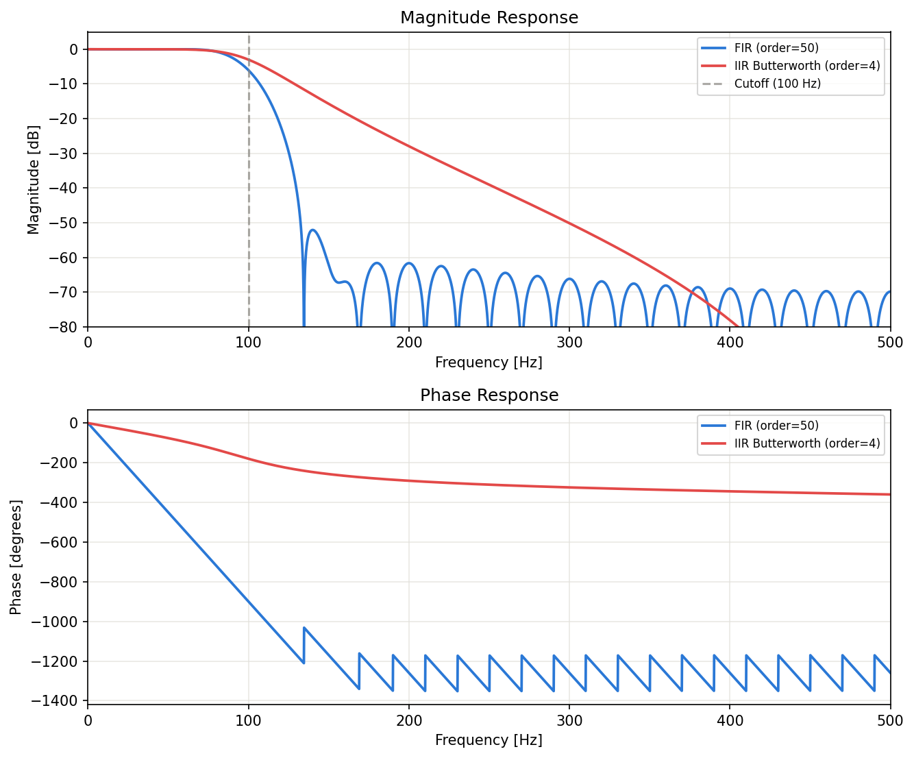
The following code designs a lowpass filter with 100 Hz cutoff frequency using both FIR and IIR approaches, and compares their frequency responses.
import numpy as np
import matplotlib.pyplot as plt
from scipy import signal

# --- Parameters ---
fs = 1000       # Sampling frequency [Hz]
fc = 100        # Cutoff frequency [Hz]
nyq = fs / 2    # Nyquist frequency

# --- FIR filter design (window method) ---
fir_order = 50
fir_coeff = signal.firwin(fir_order + 1, fc / nyq)

# --- IIR filter design (4th-order Butterworth) ---
iir_order = 4
iir_sos = signal.butter(iir_order, fc / nyq, output='sos')
iir_ba = signal.butter(iir_order, fc / nyq, output='ba')  # tf form, used for group delay

# --- Frequency response ---
w_fir, h_fir = signal.freqz(fir_coeff, worN=8192, fs=fs)
w_iir, h_iir = signal.sosfreqz(iir_sos, worN=8192, fs=fs)

# --- Plot ---
fig, axes = plt.subplots(2, 1, figsize=(10, 8))

# Magnitude response
axes[0].plot(w_fir, 20 * np.log10(np.abs(h_fir) + 1e-12), label=f'FIR (order={fir_order})')
axes[0].plot(w_iir, 20 * np.log10(np.abs(h_iir) + 1e-12), label=f'IIR Butterworth (order={iir_order})')
axes[0].set_xlabel('Frequency [Hz]')
axes[0].set_ylabel('Magnitude [dB]')
axes[0].set_title('Magnitude Response')
axes[0].set_xlim(0, 500)
axes[0].set_ylim(-80, 5)
axes[0].axvline(fc, color='gray', linestyle='--', alpha=0.5, label=f'Cutoff ({fc} Hz)')
axes[0].legend()
axes[0].grid(True, alpha=0.3)

# Phase response
angles_fir = np.unwrap(np.angle(h_fir))
angles_iir = np.unwrap(np.angle(h_iir))
axes[1].plot(w_fir, np.degrees(angles_fir), label=f'FIR (order={fir_order})')
axes[1].plot(w_iir, np.degrees(angles_iir), label=f'IIR Butterworth (order={iir_order})')
axes[1].set_xlabel('Frequency [Hz]')
axes[1].set_ylabel('Phase [degrees]')
axes[1].set_title('Phase Response')
axes[1].set_xlim(0, 500)
axes[1].legend()
axes[1].grid(True, alpha=0.3)

plt.tight_layout()
plt.savefig('fir_iir_magnitude_phase.png', dpi=150, bbox_inches='tight')
plt.show()
Numerical Verification: Magnitude Response Comparison
We actually ran the code above and compared attenuation at several frequencies.
import numpy as np
from scipy import signal

fs, fc, nyq = 1000, 100, 500
fir_coeff = signal.firwin(51, fc / nyq)
iir_sos = signal.butter(4, fc / nyq, output='sos')
w_fir, h_fir = signal.freqz(fir_coeff, worN=8192, fs=fs)
w_iir, h_iir = signal.sosfreqz(iir_sos, worN=8192, fs=fs)

def mag_db(h):
    return 20 * np.log10(np.abs(h) + 1e-300)

for f in [50, 100, 120, 150, 200, 300, 500]:
    idx_fir = np.argmin(np.abs(w_fir - f))
    idx_iir = np.argmin(np.abs(w_iir - f))
    print(f"f={f:4d}Hz  FIR={mag_db(h_fir)[idx_fir]:8.3f} dB   IIR={mag_db(h_iir)[idx_iir]:8.3f} dB")
Results:
| Frequency [Hz] | FIR (order 50) [dB] | IIR Butterworth (order 4) [dB] |
|---|---|---|
| 50 | −0.014 | −0.014 |
| 100 (cutoff) | −6.041 | −3.006 |
| 120 | −22.123 | −7.678 |
| 150 | −62.292 | −15.755 |
| 200 | −61.661 | −27.969 |
| 300 | −66.177 | −50.154 |
| 500 | −69.854 | −336.440 |
At exactly the 100 Hz cutoff, the IIR Butterworth attenuation is precisely \(-3.01\)
dB (as guaranteed by its design definition), while the FIR filter (firwin default, Hamming window) drops slightly further to \(-6.04\)
dB. Searching for the actual \(-3\)
dB point, we find \(91.9\)
Hz for FIR and \(99.9\)
Hz for IIR — the IIR filter lands closer to the design target of 100Hz. This is because signal.butter uses an analytic design formula that guarantees the cutoff location, whereas the firwin window method is only an approximation.
The transition-band sharpness tells the opposite story: the \(-40\) dB point is \(129.8\) Hz for FIR vs \(254.3\) Hz for IIR, and the \(-60\) dB point is \(133.8\) Hz for FIR vs \(340.6\) Hz for IIR. At these orders, FIR (order 50) rolls off far more sharply than IIR (order 4) — but the FIR stopband attenuation plateaus and oscillates around \(-60\) to \(-85\) dB (a consequence of the Hamming window’s sidelobe level), whereas IIR keeps decreasing monotonically, reaching \(-336\) dB at 500Hz (a 4th-order Butterworth falls off monotonically at \(-24\) dB/octave).
Numerical Verification: FIR vs IIR Order Trade-off (Matched Specifications)
We quantitatively verified the claim in the comparison table — “FIR needs high order, IIR achieves sharp characteristics with low order” — under a common design specification: passband edge at \(100\)
Hz (ripple within \(1\)
dB), stopband edge at \(150\)
Hz (attenuation of at least \(60\)
dB). We found the minimum order meeting this spec using scipy.signal.buttord / cheb1ord (IIR) and scipy.signal.kaiserord (FIR, Kaiser window).
import numpy as np
from scipy import signal

fs, nyq = 1000, 500
fp, fst, gpass, gstop = 100, 150, 1, 60

n_butter, wn_butter = signal.buttord(fp / nyq, fst / nyq, gpass, gstop)
n_cheby, wn_cheby = signal.cheb1ord(fp / nyq, fst / nyq, gpass, gstop)
numtaps, beta = signal.kaiserord(gstop, (fst - fp) / nyq)

print("Butterworth minimum order:", n_butter)
print("Chebyshev I minimum order:", n_cheby)
print("Kaiser-window FIR taps:", numtaps)
Results:
| Design method | Order (taps) needed | Measured @100Hz | Measured @150Hz |
|---|---|---|---|
| Butterworth (IIR) | order 17 | −0.992 dB | −60.59 dB |
| Chebyshev I (IIR) | order 9 | meets spec | meets spec |
| Kaiser-window FIR | 74 taps (order 73) | −0.009 dB | −63.54 dB |
Under the identical specification, FIR requires roughly 4x or more the order of IIR (Butterworth) — 73rd order vs 17th order. An equiripple design (Chebyshev I) needs even fewer, just 9th order. This is the quantitative confirmation of the “filter order” trade-off noted in the comparison table. Order translates directly into multiply-accumulate operations (computational cost), so this is where IIR’s real-time advantage comes from.
Phase and Group Delay Discussion
The key differences visible in the plots above:
- FIR filter: Phase varies linearly with frequency in the passband (linear phase). This means constant group delay, preserving the temporal shape of pulse waveforms.
- IIR filter: Phase varies nonlinearly. Phase change becomes steep near cutoff, with group delay varying by frequency. However, zero-phase filtering is achievable using
filtfilt.
Numerical Verification: Group Delay Comparison
We computed the group delay of both filters with scipy.signal.group_delay.
import numpy as np
from scipy import signal

fs, fc, nyq = 1000, 100, 500
fir_coeff = signal.firwin(51, fc / nyq)
iir_ba = signal.butter(4, fc / nyq, output='ba')

w_gd_fir, gd_fir = signal.group_delay((fir_coeff, [1.0]), w=4096, fs=fs)
w_gd_iir, gd_iir = signal.group_delay(iir_ba, w=4090, fs=fs)  # 4090: avoid the singularity just below Nyquist

print("FIR group delay mean/std (0-80Hz):", np.mean(gd_fir[w_gd_fir < 80]), np.std(gd_fir[w_gd_fir < 80]))
for f in [10, 50, 90, 100, 110, 150]:
    idx = np.argmin(np.abs(w_gd_iir - f))
    print(f"IIR group delay @{f}Hz:", gd_iir[idx], "samples")
Results:
- FIR group delay: mean \(25.0\) samples across \(0\) –\(80\) Hz, standard deviation \(8.9\times10^{-15}\) — constant to within numerical noise
- IIR group delay (frequency-dependent): \(4.04\) samples at \(10\) Hz, \(4.66\) at \(50\) Hz, \(6.52\) at \(90\) Hz (peak, near cutoff), \(6.29\) at \(100\) Hz, \(5.53\) at \(110\) Hz, \(2.61\) at \(150\) Hz
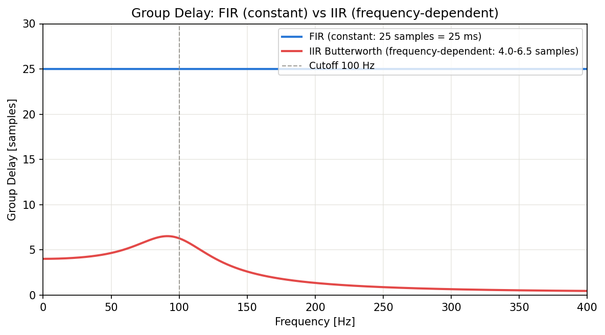
The IIR group delay peaks (at \(6.5\) samples) just below the cutoff (\(90\) Hz), then decreases on either side — a non-monotonic shape. This is because the transfer function’s poles are complex-conjugate pairs, and phase changes rapidly near their argument. Passing pulse-like or transient waveforms through an IIR filter distorts the rising edge due to this frequency-dependent delay difference (appearing as pre-echo/post-echo). This contrasts with the FIR group delay, which is constant regardless of frequency (standard deviation is effectively zero).
Practical Selection Guidelines
- Faithful waveform reproduction needed (ECG, audio, seismic) → FIR (linear phase)
- Real-time processing with low computational cost → IIR (low order)
- Absolute stability guarantee required → FIR
- Reproduce analog filter characteristics → IIR (bilinear transform)
Recent Research: Differentiable IIR Filters and Learned Stability Constraints
In recent years, differentiable digital signal processing (DDSP), which treats FIR/IIR filter coefficients as learnable neural-network parameters, has advanced rapidly in the music and speech synthesis field. A 2024 review by Hayes et al. systematically surveys multiple approaches to optimizing IIR filter coefficients via gradient descent (time-domain BPTT, frequency-sampling methods, cascaded second-order-section constructions, and more), and identifies how to satisfy — during training — the very stability constraint we proved in Eqs.(12)-(15) of this article (“all poles must lie inside the unit circle”) as a central practical challenge.
More concretely, a 2025 paper by Malek et al. (presented at DAFx25) applies Kolmogorov-Arnold Networks (KANs) to optimize biquad (second-order IIR section) coefficients, proposing a method that generates coefficients via a neural network while preserving the constraint that poles remain inside the unit circle. With naive neural-network coefficient prediction, poles can drift outside the unit circle early in training or due to gradient noise, causing divergence; the common remedy is reparameterization (e.g., expressing poles in polar form \((r,\theta)\) and constraining \(r<1\) via a sigmoid). The stability condition derived in this article remains the underlying constraint even in these state-of-the-art learning-based methods.
Related Articles
- Frequency Characteristics of the EMA Filter - EMA is a type of IIR filter and the most basic first-order IIR filter.
- Fast Fourier Transform (FFT): Theory and Python Implementation - Detailed explanation of FFT used for analyzing filter frequency characteristics.
- Moving Average Filters Compared: SMA, WMA, and EMA in Python - Compares types and characteristics of moving average filters, the most basic form of FIR filters.
- Low-Pass Filter Design and Comparison - Compares frequency responses of IIR filters including Butterworth and Chebyshev.
- Kalman Filter: Theory and Python Implementation - Explains filtering based on state-space models.
- Notch Filter Design and Python Implementation - IIR filter application for power line noise removal.
- Adaptive Filters (LMS/RLS): Theory and Python Implementation - An extension of FIR/IIR filters that automatically updates filter coefficients based on the input signal.
- LMS and NLMS Adaptive Algorithms: Theory and Python Implementation - The canonical adaptive filter built on an FIR structure; complements this article on how FIR characteristics relate to convergence.
- Convolution and Correlation: Theory and Python Implementation - Foundational theory behind FIR filtering — convolution with a coefficient sequence.
- Bandpass Filter Design: Theory and Python Implementation - Practical embodiment of the FIR vs IIR trade-off: linear phase (FIR) vs sharper roll-off (IIR) in band-pass design.
- Chebyshev Filter Design: Theory and Python Implementation - Equiripple IIR with sharper transition than Butterworth; contrast with FIR equiripple design (Parks-McClellan).
- Bessel Filter: Theory and Python Implementation - IIR with maximally flat group delay; the natural counterpoint to FIR’s strictly linear phase when minimizing phase distortion.
- Filter Design Selection Guide: 3 axes and characteristic comparison — Use this hub to position FIR vs IIR against alternatives during selection.
- Multirate Signal Processing in Python: Decimation, Interpolation, and Polyphase Filters - Anti-aliasing FIR filters made efficient via polyphase decomposition — a domain where FIR linear phase pays off in practice.
- Z-Transform and Digital Filter Transfer Functions - The theoretical foundation that expresses FIR/IIR difference equations as transfer functions \(H(z)\) and reads stability and frequency response from pole-zero placement.
References
- Oppenheim, A. V., & Schafer, R. W. (2009). Discrete-Time Signal Processing (3rd ed.). Prentice Hall.
- Parks, T. W., & Burrus, C. S. (1987). Digital Filter Design. Wiley.
- SciPy Signal Processing documentation
- Hayes, B., Shier, J., Fazekas, G., McPherson, A., & Saitis, C. (2024). “A review of differentiable digital signal processing for music and speech synthesis.” Frontiers in Signal Processing, 3. https://doi.org/10.3389/frsip.2023.1284100
- Malek, A., Schulz, D., & Wuebbelmann, F. (2025). “Biquad coefficients optimization via Kolmogorov-Arnold Networks.” Proceedings of the 28th International Conference on Digital Audio Effects (DAFx25). https://www.dafx.de/paper-archive/2025/DAFx25_paper_10.pdf