Introduction
Genetic Algorithm (GA) is a metaheuristic optimization technique inspired by biological evolution. It repeatedly applies selection, crossover, and mutation to a population of candidate solutions to search for optima of an objective function.
GA is a gradient-free black-box optimization method applicable to multimodal functions and discrete optimization problems.
Algorithm Overview
The basic GA flow is:
- Initialization: Randomly generate \(N\) individuals
- Fitness evaluation: Compute objective function for each individual
- Selection: Select high-fitness individuals as parents
- Crossover: Generate offspring from parent pairs
- Mutation: Modify genes of individuals with some probability
- Replacement: Form the next generation
- Repeat steps 2-6 until convergence
Selection
Tournament Selection
Randomly pick \(k\) individuals from the population and select the one with the best fitness. \(k\) is called the tournament size; larger values increase selection pressure.
\[P(\text{best individual selected}) = 1 - \left(1 - \frac{1}{N}\right)^k \tag{1}\]Roulette Wheel Selection
Select individuals with probability proportional to fitness. The selection probability for individual \(i\) is:
\[P(i) = \frac{f(x_i)}{\sum_{j=1}^{N} f(x_j)} \tag{2}\]where \(f(x_i)\) is the fitness of individual \(i\) . For minimization problems, a fitness transformation (e.g., \(f' = f_{\max} - f\) ) is needed.
Crossover
BLX-\(\alpha\) Crossover (for Real-Valued Optimization)
For continuous optimization, BLX-\(\alpha\) crossover is widely used. When generating a child from parents \(p_1, p_2\) , each dimension \(d\) is computed as:
\[c_d = U\left[\min(p_{1,d}, p_{2,d}) - \alpha \cdot I_d, \; \max(p_{1,d}, p_{2,d}) + \alpha \cdot I_d\right] \tag{3}\]where \(I_d = |p_{1,d} - p_{2,d}|\) , \(U[a, b]\) is the uniform distribution, and \(\alpha\) is typically 0.5.
Mutation
Gaussian Mutation
For continuous optimization, adding Gaussian noise is the standard mutation approach:
\[x'_d = x_d + \mathcal{N}(0, \sigma^2) \tag{4}\]\(\sigma\) controls mutation strength. Adaptive mutation that decreases \(\sigma\) over generations is also effective.
The Schema Theorem: Why GA Works
We have introduced selection, crossover, and mutation as separate operators. But why does combining them lead to efficient search for good solutions? Holland’s (1975) Schema Theorem is the first rigorous answer to this question.
Schemata and the Building Block Hypothesis
Representing an individual of length \(l\) as a binary string in \(\{0,1\}^l\) , a schema \(H\) is a template that assigns \(0\) , \(1\) , or a wildcard \(*\) to each position. For example, with \(l=6\) , \(H = 1{*}1{*}{*}0\) represents the set of individuals whose 1st bit is 1, 3rd bit is 1, and 6th bit is 0 (the remaining 3 bits are free, so \(2^3=8\) individuals match).
Two quantities characterize a schema:
- Order \(o(H)\) : the number of fixed (non-wildcard) bits (here \(o(H)=3\) )
- Defining length \(\delta(H)\) : the distance between the first and last fixed bit positions (here \(6-1=5\) )
Let \(m(H,t)\) denote the number of individuals in generation \(t\) matching schema \(H\) , \(f(H,t)\) its average fitness, and \(\bar f(t)\) the average fitness of the whole population. The idea that a GA implicitly evaluates a huge number of overlapping schemata in parallel, even though it only explicitly evaluates individuals, is called implicit parallelism.
Growth of Schema Count under Selection
Under fitness-proportional selection, individual \(x_i\) is chosen in a single draw with probability \(p_i = f(x_i)/(N\bar f)\) from Eq.(2). Over \(N\) draws (with replacement), the expected number of copies of \(x_i\) is \(Np_i = f(x_i)/\bar f\) . Summing this expected count over all individuals matching schema \(H\) gives
\[ m(H,t+1)\big|_{\text{selection only}} \;=\; \sum_{i:\, x_i \in H} \frac{f(x_i)}{\bar f(t)} \;=\; m(H,t)\cdot\frac{f(H,t)}{\bar f(t)} \tag{6} \]Considering selection alone, the schema count \(m(H,t)\) grows or shrinks geometrically with ratio \(f(H,t)/\bar f(t)\) . If this ratio is roughly constant at \(1+c\) across generations, then \(m(H,t) \approx m(H,0)(1+c)^t\) — an above-average schema grows exponentially.
Disruption Probability under Crossover
Single-point crossover picks one of \(l-1\) possible cut points uniformly at random along a length-\(l\) string. If the cut point falls inside the span defined by \(H\) ’s fixed bits (of length \(\delta(H)\) ), the offspring may inherit mismatched fragments from the two parents and lose the match to \(H\) . If the cut point falls outside that span, \(H\) is always preserved. Assuming crossover occurs with probability \(p_c\) , the disruption probability is bounded above by
\[ P(\text{disrupted} \mid \text{crossover}) \;\le\; \frac{\delta(H)}{l-1} \tag{7} \](this ignores the cases where a cut inside the span happens to still preserve the match, so it is a pessimistic upper bound on disruption). Hence the survival probability after crossover is \(P(\text{survives}) \ge 1 - p_c\,\delta(H)/(l-1)\) .
Disruption Probability under Mutation
Under bit-flip mutation, each bit flips independently with probability \(p_m\) . The probability that all \(o(H)\) fixed bits of \(H\) remain unchanged is \((1-p_m)^{o(H)}\) . Applying Bernoulli’s inequality \((1-p_m)^n \ge 1-np_m\) (valid for \(p_m\in[0,1]\) and any non-negative integer \(n\) ) with \(n=o(H)\) gives
\[ P(\text{survives}) \;=\; (1-p_m)^{o(H)} \;\ge\; 1-o(H)\,p_m \tag{8} \]The Schema Theorem (Combined)
Treating the three effects of selection, crossover, and mutation as approximately independent and multiplying them together yields Holland’s Schema Theorem:
\[ m(H,t+1) \;\ge\; m(H,t)\cdot\frac{f(H,t)}{\bar f(t)}\cdot\left[1-p_c\frac{\delta(H)}{l-1}-o(H)p_m\right] \tag{9} \](Simply adding the crossover and mutation disruption probabilities is a first-order approximation that ignores the higher-order cross term \(p_c p_m\) , valid when both are small.)
This inequality states that “short (small \(\delta(H)\) ), low-order (small \(o(H)\) ), above-average schemata (\(f(H)/\bar f>1\) )” — building blocks — receive an exponentially growing share of the population across generations. The hypothesis that a GA searches globally by combining these building blocks via crossover is the Building Block Hypothesis. Note that Eq.(9) is only a lower bound: the crossover disruption probability is a pessimistic upper bound, the mutation survival probability is a first-order approximation, and independence among the three operators is itself an approximation.
Experimental Verification: Growth of Building Blocks
We check numerically how well Eq.(9) holds in an actual simulation. Individuals are binary strings of length \(l=20\) , and we track the count \(m(H,t)\) of individuals matching schema \(H = 1111{*}{*}\cdots{*}\) (first 4 bits equal to 1, so \(o(H)=4\) , \(\delta(H)=3\) ). Fitness is \(f(x)=\sum_i x_i\) (the number of 1-bits), so individuals matching \(H\) have a higher average fitness because their first 4 bits are guaranteed 1s. We run the GA with roulette-wheel selection, single-point crossover (\(p_c=0.7\) ), and bit-flip mutation (\(p_m=0.01\) ).
import numpy as np

L = 20          # individual length l
O_H = 4         # order o(H) of schema H: number of fixed bits
DELTA_H = 3     # defining length delta(H): first 4 bits (positions 0-3), so 3
N = 200         # population size
PC = 0.7        # crossover rate
PM = 0.01       # mutation rate
GENERATIONS = 30
TRIALS = 200    # trials for expectation estimate

def matches_schema(pop):
    """Matches schema H = 1111************** (first 4 bits equal 1)"""
    return np.all(pop[:, :O_H] == 1, axis=1)

def run_trial(seed):
    rng = np.random.default_rng(seed)
    pop = rng.integers(0, 2, size=(N, L))

    m_actual = []
    rhs_bound = []

    for t in range(GENERATIONS):
        fitness = pop.sum(axis=1).astype(float)
        f_bar = fitness.mean()

        match = matches_schema(pop)
        m_t = match.sum()
        m_actual.append(m_t)
        f_H = fitness[match].mean() if m_t > 0 else 0.0

        selection_term = (f_H / f_bar) if f_bar > 0 else 0.0
        disruption_term = max(1 - PC * DELTA_H / (L - 1) - O_H * PM, 0.0)
        rhs_bound.append(m_t * selection_term * disruption_term)

        # --- generational step: roulette selection -> single-point crossover -> mutation ---
        probs = fitness / fitness.sum() if fitness.sum() > 0 else np.ones(N) / N
        parent_idx = rng.choice(N, size=N, p=probs)
        parents = pop[parent_idx]

        children = parents.copy()
        for i in range(0, N - 1, 2):
            if rng.random() < PC:
                point = rng.integers(1, L)
                children[i, point:], children[i + 1, point:] = (
                    parents[i + 1, point:].copy(),
                    parents[i, point:].copy(),
                )

        mutate_mask = rng.random((N, L)) < PM
        children = np.where(mutate_mask, 1 - children, children)
        pop = children

    match = matches_schema(pop)
    m_actual.append(match.sum())
    return np.array(m_actual), np.array(rhs_bound)

all_m, all_rhs = [], []
for trial in range(TRIALS):
    m_actual, rhs_bound = run_trial(seed=trial)
    all_m.append(m_actual)
    all_rhs.append(rhs_bound)

all_m, all_rhs = np.array(all_m), np.array(all_rhs)
mean_m, mean_rhs = all_m.mean(axis=0), all_rhs.mean(axis=0)

print(f"mean m(H,0) = {mean_m[0]:.3f} (theoretical N*0.5^{O_H} = {N*0.5**O_H:.3f})")
print(f"mean m(H,{GENERATIONS}) = {mean_m[-1]:.3f}")
print(f"generations violating the bound (mean-based): {np.sum(mean_m[1:] < mean_rhs)}/{GENERATIONS}")
violations = np.sum(all_m[:, 1:] < all_rhs)
print(f"per-trial bound violation rate: {violations}/{all_m[:,1:].size} = {violations/all_m[:,1:].size*100:.2f}%")
Averaged over 200 trials, the results were:
- The mean \(m(H,0)\) in the initial generation was 12.68 (6.3% of the 200 individuals, matching the theoretical value \(N\times0.5^4=12.5\) )
- After 30 generations, the mean \(m(H,30)\) grew to 80.64 (40.3% of the population) — over 6.4 times the initial count
- Looking at the generation-averaged series, the lower bound in Eq.(9) held in all 30 generations (0/30 violations)
- At the level of individual trials (one trial = one full GA run), the bound was violated in 890/6000 = 14.83% of cases. This confirms the theoretical nature of the Schema Theorem: it is an inequality about an expectation, and individual stochastic trials can and do fall below it.
This quantitatively confirms that short, low-order, above-average schemata grow within the population across generations, exactly as the Schema Theorem predicts.
The No Free Lunch Theorem: GA Is Not a Universal Optimizer
The Schema Theorem explains why GA works, but only when the fitness landscape has structure that decomposes into building blocks. Wolpert and Macready’s (1997) No Free Lunch (NFL) theorem proves the following:
Averaged over the set of all possible objective functions, any two black-box optimization algorithms (including GA) perform identically. In other words, no algorithm is on average better than any other across all possible problems.
This means that GA appears to outperform random search only because real-world problems are not arbitrary random objective functions — they tend to have structure that aligns with GA’s implicit assumptions (decomposability into building blocks, local smoothness of the fitness landscape, and so on). If an objective function is adversarial to GA’s assumptions, or genuinely close to random, GA can perform no better than — or worse than — random search. Anyone adopting a GA should always ask “does this problem have building-block-like structure?” GA is never a universal optimization algorithm.
Python Implementation: Rastrigin Function Optimization
The Rastrigin function is a multimodal benchmark with global minimum \(f(\mathbf{0}) = 0\) :
\[f(\mathbf{x}) = 10n + \sum_{i=1}^{n} \left[x_i^2 - 10\cos(2\pi x_i)\right] \tag{5}\]import numpy as np
import matplotlib.pyplot as plt
def rastrigin(x):
"""Rastrigin function (batch-safe: the constant term uses x.shape[-1], the dimensionality)"""
return 10 * x.shape[-1] + np.sum(x**2 - 10 * np.cos(2 * np.pi * x), axis=-1)
class GeneticAlgorithm:
def __init__(self, dim, pop_size=100, bounds=(-5.12, 5.12),
crossover_rate=0.8, mutation_rate=0.1, mutation_sigma=0.5,
tournament_size=3):
self.dim = dim
self.pop_size = pop_size
self.bounds = bounds
self.crossover_rate = crossover_rate
self.mutation_rate = mutation_rate
self.mutation_sigma = mutation_sigma
self.tournament_size = tournament_size
def initialize(self):
"""Generate random initial population"""
low, high = self.bounds
return np.random.uniform(low, high, (self.pop_size, self.dim))
def tournament_selection(self, population, fitness):
"""Tournament selection"""
indices = np.random.randint(0, self.pop_size, size=self.tournament_size)
best = indices[np.argmin(fitness[indices])]
return population[best]
def blx_alpha_crossover(self, parent1, parent2, alpha=0.5):
"""BLX-alpha crossover"""
low = np.minimum(parent1, parent2) - alpha * np.abs(parent1 - parent2)
high = np.maximum(parent1, parent2) + alpha * np.abs(parent1 - parent2)
child = np.random.uniform(low, high)
return np.clip(child, *self.bounds)
def gaussian_mutation(self, individual):
"""Gaussian mutation"""
mask = np.random.random(self.dim) < self.mutation_rate
noise = np.random.normal(0, self.mutation_sigma, self.dim)
individual[mask] += noise[mask]
return np.clip(individual, *self.bounds)
def run(self, objective, max_generations=200):
"""Run GA"""
population = self.initialize()
best_history = []
for gen in range(max_generations):
fitness = objective(population)
best_idx = np.argmin(fitness)
best_history.append(fitness[best_idx])
new_population = [population[best_idx].copy()] # Elitism
while len(new_population) < self.pop_size:
p1 = self.tournament_selection(population, fitness)
p2 = self.tournament_selection(population, fitness)
if np.random.random() < self.crossover_rate:
child = self.blx_alpha_crossover(p1, p2)
else:
child = p1.copy()
child = self.gaussian_mutation(child)
new_population.append(child)
population = np.array(new_population[:self.pop_size])
fitness = objective(population)
best_idx = np.argmin(fitness)
return population[best_idx], fitness[best_idx], best_history
# --- Run ---
np.random.seed(42)
ga = GeneticAlgorithm(dim=10, pop_size=200)
best_solution, best_fitness, history = ga.run(rastrigin, max_generations=300)
print(f"Best fitness: {best_fitness:.6f}")
print(f"Best solution: {best_solution[:3]}... (first 3 dimensions)")
# --- Convergence plot ---
plt.figure(figsize=(10, 5))
plt.plot(history, color="#2a78d6", linewidth=2)
plt.xlabel('Generation')
plt.ylabel('Best Fitness')
plt.title('GA Convergence on Rastrigin Function (10D)')
plt.yscale('log')
plt.grid(True, alpha=0.25)
plt.gca().spines[["top", "right"]].set_visible(False)
plt.tight_layout()
plt.savefig("ga_convergence.png", dpi=150)
plt.show()
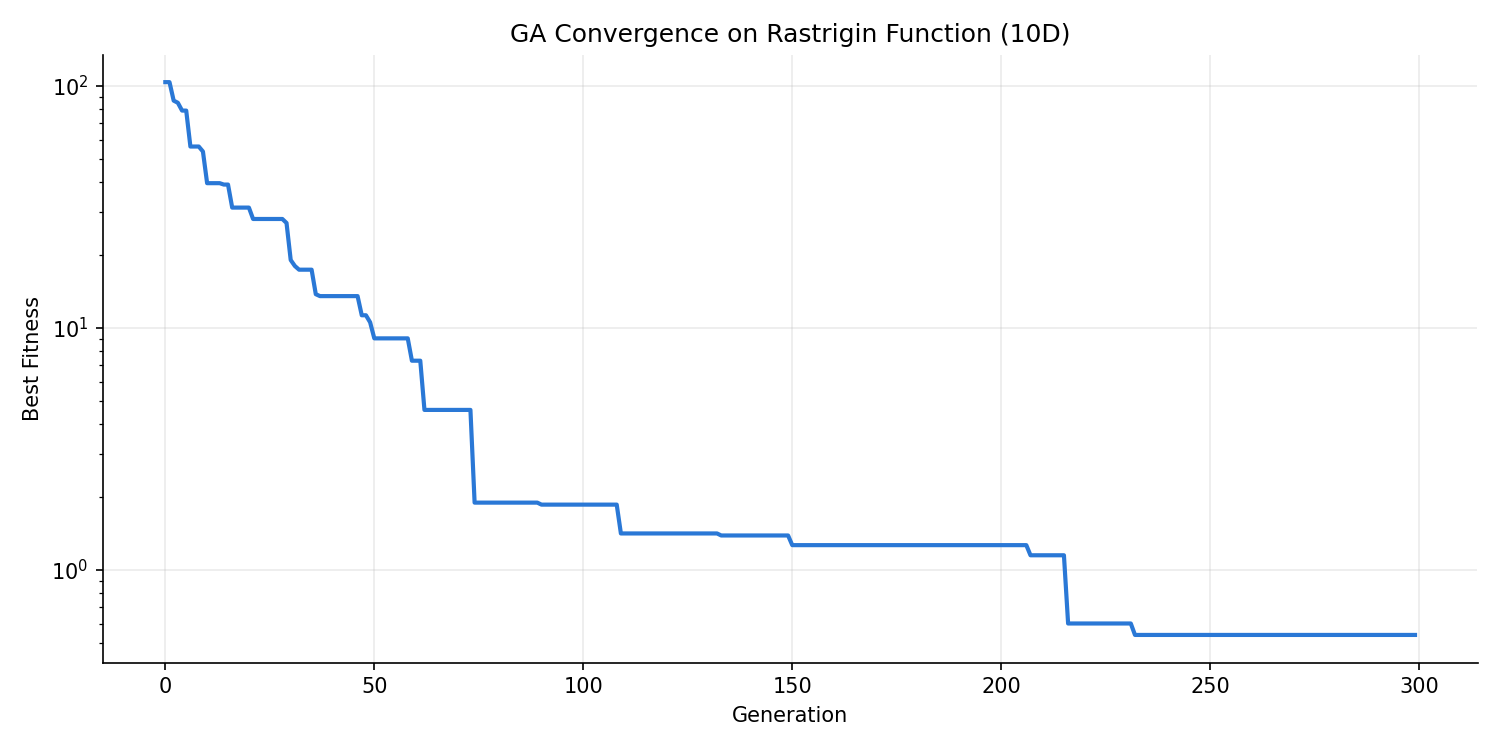
Running the code above, the best fitness starts at 103.6658 at generation 0 and drops to 0.538853 after 300 generations, converging close to the global minimum \(f(\mathbf{0})=0\) of the 10-dimensional Rastrigin function. The best solution found is \([0.0322, -0.0124, -0.0085, \ldots]\) , with every dimension clustered near zero — evidence that the GA finds the global basin rather than getting stuck in one of the function’s many local optima.
Premature Convergence and Diversity: The Selection Pressure Trade-off
What Is Premature Convergence?
If selection pressure is too strong, population diversity is lost within a handful of generations, and the whole population collapses onto a local optimum (or simply the best individual found early on) before the global optimum is reached. This is called premature convergence. Increasing the tournament size \(k\) in tournament selection raises the probability that the best individual is selected — as Eq.(1) shows — which increases selection pressure but also speeds up the loss of diversity.
Experimental Verification: Diversity Decay under Selection Alone
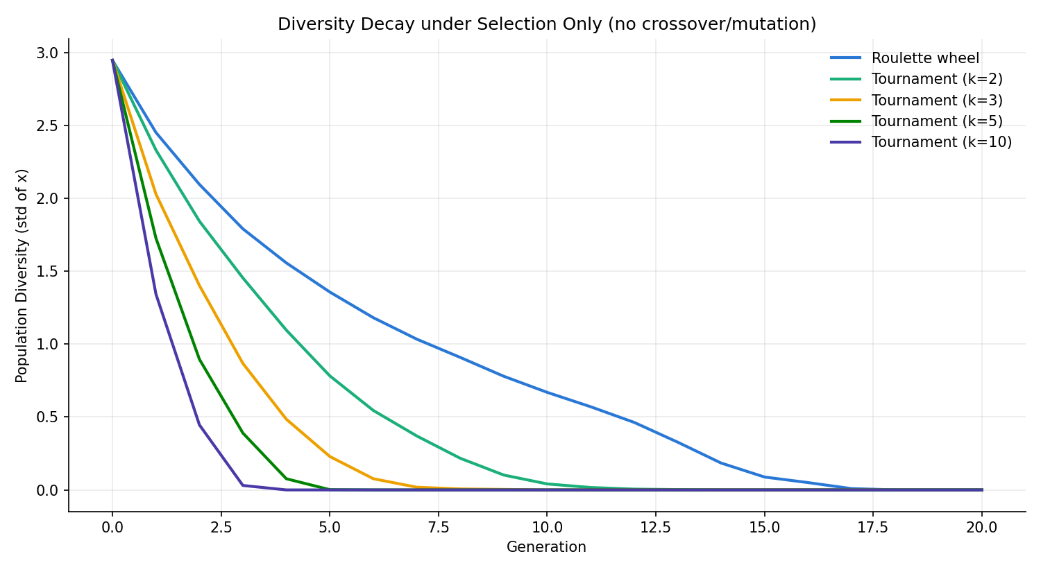
To isolate the effect of selection pressure on diversity, we apply selection only — no crossover, no mutation — repeatedly. Starting from a population of 200 individuals uniformly distributed over the 1-D Rastrigin function, we compare roulette-wheel selection against tournament selection (\(k=2,3,5,10\) ) and track how the population standard deviation (a diversity measure) decays over generations.
import numpy as np

N = 200
GENERATIONS = 40
TRIALS = 100
BOUNDS = (-5.12, 5.12)

def rastrigin_1d(x):
    return 10 + x**2 - 10 * np.cos(2 * np.pi * x)

def roulette_select(pop, fitness, rng):
    """Roulette-wheel selection (minimization, so transform f' = fmax - f)"""
    f_prime = fitness.max() - fitness
    total = f_prime.sum()
    probs = f_prime / total if total > 0 else np.ones(N) / N
    idx = rng.choice(N, size=N, p=probs)
    return pop[idx]

def tournament_select(pop, fitness, rng, k):
    """Tournament selection with tournament size k"""
    idx = rng.integers(0, N, size=(N, k))
    best = idx[np.arange(N), np.argmin(fitness[idx], axis=1)]
    return pop[best]

def run_trial(method, seed, k=None):
    rng = np.random.default_rng(seed)
    pop = rng.uniform(*BOUNDS, size=N)
    stds = [pop.std()]
    for gen in range(GENERATIONS):
        fitness = rastrigin_1d(pop)
        pop = roulette_select(pop, fitness, rng) if method == "roulette" \
            else tournament_select(pop, fitness, rng, k)
        stds.append(pop.std())
    return np.array(stds)

methods = [("roulette", None), ("tournament", 2), ("tournament", 3),
           ("tournament", 5), ("tournament", 10)]

for method, k in methods:
    all_stds = np.array([run_trial(method, seed=t, k=k) for t in range(TRIALS)])
    mean_stds = all_stds.mean(axis=0)
    half = mean_stds[0] / 2
    gen_half = next((t + (mean_stds[t] - half) / (mean_stds[t] - mean_stds[t + 1])
                      for t in range(len(mean_stds) - 1)
                      if mean_stds[t] >= half > mean_stds[t + 1]), None)
    gen_1pct = next((t for t, s in enumerate(mean_stds) if s < mean_stds[0] * 0.01), None)
    label = f"{method}(k={k})" if k else method
    print(f"{label:20s} half-life(gen)={gen_half}  1%-reached gen={gen_1pct}")
Averaged over 100 trials (initial standard deviation 2.9459), the results were:
| Selection method | Diversity half-life (generations) | Generation diversity drops below 1% of initial |
|---|---|---|
| Roulette wheel | 4.42 | 17 |
| Tournament (\(k=2\) ) | 2.95 | 11 |
| Tournament (\(k=3\) ) | 1.89 | 7 |
| Tournament (\(k=5\) ) | 1.31 | 5 |
| Tournament (\(k=10\) ) | 0.92 | 4 |
Roulette-wheel selection takes about 4.4 generations for diversity to halve, whereas tournament selection with \(k=10\) halves diversity in under one generation and drives the population to near-total convergence (diversity below 1%) in just 4 generations. Stronger selection pressure converges faster, but this comes at the cost of homogenizing the population before it has explored the multimodal landscape thoroughly. The figure below visualizes this diversity decay across the five selection methods.
In practice, premature convergence is mitigated by tuning selection pressure alongside elitism, by niching/sharing techniques that actively preserve diversity, or by tuning the mutation rate, which we turn to next.
The Crossover-Mutation Rate Trade-off
The mutation rate \(p_m\) is one of the most important hyperparameters governing the trade-off between diversity maintenance and search efficiency.
- If \(p_m\) is too low, selection and crossover alone cannot replenish lost diversity, and the population homogenizes prematurely, getting stuck in local optima (the same mechanism as premature convergence above)
- If \(p_m\) is too high, good gene values are also destroyed at random, and the GA effectively degenerates into random search, unable to exploit the information accumulated by selection and crossover
Experimental Verification: Mutation Rate vs. Final Solution Quality and Diversity
We extend the Rastrigin optimizer above so the random generator can be injected externally (an rng argument) and each generation’s population diversity is recorded as diversity_history. We then sweep the mutation rate \(p_m\)
from \(0\)
to \(1.0\)
and average, over 30 random seeds, the best fitness and diversity of the final (150th) generation.
import numpy as np

def rastrigin(x):
    """Rastrigin function (batch-safe: the constant term uses x.shape[-1], the dimensionality)"""
    return 10 * x.shape[-1] + np.sum(x**2 - 10 * np.cos(2 * np.pi * x), axis=-1)

class GeneticAlgorithm:
    def __init__(self, dim, pop_size=100, bounds=(-5.12, 5.12),
                 crossover_rate=0.8, mutation_rate=0.1, mutation_sigma=0.5,
                 tournament_size=3, rng=None):
        self.dim = dim
        self.pop_size = pop_size
        self.bounds = bounds
        self.crossover_rate = crossover_rate
        self.mutation_rate = mutation_rate
        self.mutation_sigma = mutation_sigma
        self.tournament_size = tournament_size
        self.rng = rng if rng is not None else np.random.default_rng()

    def initialize(self):
        low, high = self.bounds
        return self.rng.uniform(low, high, (self.pop_size, self.dim))

    def tournament_selection(self, population, fitness):
        indices = self.rng.integers(0, self.pop_size, size=self.tournament_size)
        best = indices[np.argmin(fitness[indices])]
        return population[best]

    def blx_alpha_crossover(self, parent1, parent2, alpha=0.5):
        low = np.minimum(parent1, parent2) - alpha * np.abs(parent1 - parent2)
        high = np.maximum(parent1, parent2) + alpha * np.abs(parent1 - parent2)
        child = self.rng.uniform(low, high)
        return np.clip(child, *self.bounds)

    def gaussian_mutation(self, individual):
        mask = self.rng.random(self.dim) < self.mutation_rate
        noise = self.rng.normal(0, self.mutation_sigma, self.dim)
        individual[mask] += noise[mask]
        return np.clip(individual, *self.bounds)

    def run(self, objective, max_generations=150):
        population = self.initialize()
        best_history = []
        diversity_history = []

        for gen in range(max_generations):
            fitness = objective(population)
            best_idx = np.argmin(fitness)
            best_history.append(fitness[best_idx])
            diversity_history.append(population.std())

            new_population = [population[best_idx].copy()]  # Elitism
            while len(new_population) < self.pop_size:
                p1 = self.tournament_selection(population, fitness)
                p2 = self.tournament_selection(population, fitness)
                if self.rng.random() < self.crossover_rate:
                    child = self.blx_alpha_crossover(p1, p2)
                else:
                    child = p1.copy()
                child = self.gaussian_mutation(child)
                new_population.append(child)

            population = np.array(new_population[:self.pop_size])

        fitness = objective(population)
        best_idx = np.argmin(fitness)
        return population[best_idx], fitness[best_idx], best_history, diversity_history

mutation_rates = [0.0, 0.01, 0.05, 0.1, 0.2, 0.4, 0.6, 0.8, 1.0]
DIM, POP, GENS, SEEDS = 5, 100, 150, 30

for mr in mutation_rates:
    finals, diversities = [], []
    for seed in range(SEEDS):
        rng = np.random.default_rng(seed * 1000 + int(mr * 100))
        ga = GeneticAlgorithm(dim=DIM, pop_size=POP, mutation_rate=mr, rng=rng)
        _, best_fitness, history, div_history = ga.run(rastrigin, max_generations=GENS)
        finals.append(best_fitness)
        diversities.append(div_history[-1])
    finals = np.array(finals)
    print(f"mutation_rate={mr:.2f}  mean final best fitness={finals.mean():.5f}  "
          f"(std={finals.std():.5f})  mean final diversity={np.mean(diversities):.5f}")
The results were:
| Mutation rate \(p_m\) | Mean final best fitness | Std. dev. | Mean final diversity |
|---|---|---|---|
| 0.00 | 2.35483 | 1.27119 | 0.61979 |
| 0.01 | 0.19900 | 0.39798 | 0.12307 |
| 0.05 | 0.03336 | 0.17857 | 0.12191 |
| 0.10 | 0.12742 | 0.48329 | 0.23791 |
| 0.20 | 0.35329 | 0.42528 | 0.44111 |
| 0.40 | 2.35655 | 0.98452 | 0.94158 |
| 0.60 | 3.61938 | 1.04975 | 1.12032 |
| 0.80 | 4.80038 | 1.25726 | 1.25964 |
| 1.00 | 5.39044 | 1.50549 | 1.34802 |
The results show a textbook U-shaped curve. At \(p_m=0\) (no mutation) the final fitness is a poor 2.35, because BLX-\(\alpha\) crossover alone cannot compensate for the resulting loss of diversity and premature convergence sets in. Increasing \(p_m\) reaches the best fitness of 0.033 around \(p_m=0.05\) , but pushing \(p_m\) further monotonically worsens performance: at \(p_m=1.0\) (every gene overwritten by Gaussian noise every generation — essentially pure random search) the mean fitness degrades to 5.39. Final diversity also increases monotonically with \(p_m\) (from 0.12 to 1.35), quantitatively confirming that the mutation rate directly controls population diversity.
Recent Research Trends (2023 and Later)
Evolutionary computation and GA have expanded well beyond classical numerical optimization. The following applications have grown in recent years; given the pace of the field, consult the primary literature for details.
- Fusion with Neural Architecture Search (NAS): Encoding a neural network’s layer structure or hyperparameters as an individual’s genome, then searching the architecture space via GA-style crossover and mutation, remains an active line of research. Discrete architecture search spaces where gradients are unavailable are a natural fit for GA, and combining this with surrogate models or multi-fidelity evaluation to reduce the cost of expensive train/validate evaluations continues to be studied.
- Comparison with CMA-ES (Covariance Matrix Adaptation Evolution Strategy): CMA-ES is an evolution strategy that adaptively updates a covariance matrix, learning the shape of the search distribution itself; it is frequently reported to be more sample-efficient than GA for continuous optimization. GA, in turn, retains the flexibility to handle discrete combinatorial structure via crossover, so the choice between the two continues to be framed around problem characteristics (continuous vs. discrete, the structure of variable interactions).
- Evolution strategies for LLM prompt optimization: Since 2023, several studies have applied evolutionary methods — having an LLM itself perform “crossover” and “mutation” on prompts, or evaluating and selecting among a discrete population of prompts — to search prompts and in-context exemplars for large language models. This is a domain where GA’s black-box optimization nature is well suited, since the discrete text space cannot be optimized via gradient backpropagation.
Given how quickly this area is evolving, consult primary sources for detailed performance comparisons and reproducibility of these applications.
Comparison with Other Methods
| Method | Population-based | Gradient-free | Discrete problems | Key feature |
|---|---|---|---|---|
| GA | Yes | Yes | Yes | Combinatorial exploration via crossover |
| CEM | Yes | Yes | Difficult | Iterative distribution update |
| PSO | Yes | Yes | Difficult | Velocity-based particle movement |
| SA | No | Yes | Yes | Probabilistic acceptance via temperature |
Related Articles
- Simulated Annealing: Theory and Python Implementation - Another metaheuristic based on temperature-driven stochastic search.
- Bayesian Optimization: Fundamentals and Python Implementation - Efficient optimization using Gaussian process surrogate models.
- From SGD to Adam: Evolution of Gradient-Based Optimization - Gradient-based optimization; GA is an alternative when gradients are unavailable.
- MPPI (Model Predictive Path Integral): A Unified View with the Cross-Entropy Method - Sampling-based control optimization.
- Cross-Entropy Method: A Practical Monte Carlo Optimization Technique - CEM is also a black-box optimizer but uses distribution updates for exploration.
- Particle Swarm Optimization (PSO) Python Implementation - Another metaheuristic based on swarm intelligence.
- Particle Swarm Optimization (PSO): Theory and Python Implementation - Updated treatment with inertia-weight scheduling; useful for contrasting velocity-update PSO with GA’s selection/crossover.
- Gaussian Process Regression: Theory and Python Implementation - GP surrogate models target expensive-evaluation problems, complementing GA’s mass-sampling strategy.
- Markov Chain Monte Carlo (MCMC): Metropolis-Hastings and Gibbs Sampling - Probabilistic-sampling counterpart to GA’s selection/crossover; same probabilistic-modeling framework, different search strategy.
- Monte Carlo Optimization Methods Comparison (CEM/SA/GA/MPPI/PSO) - Hub article comparing five Monte Carlo optimizers including GA under a common sample/evaluate/update skeleton, with guidance on when evolutionary methods are preferable.
References
- Holland, J. H. (1975). Adaptation in Natural and Artificial Systems. University of Michigan Press.
- Goldberg, D. E. (1989). Genetic Algorithms in Search, Optimization, and Machine Learning. Addison-Wesley.
- Eshelman, L. J., & Schaffer, J. D. (1993). “Real-coded genetic algorithms and interval-schemata”. Foundations of Genetic Algorithms, 2, 187-202.
- Wolpert, D. H., & Macready, W. G. (1997). “No free lunch theorems for optimization”. IEEE Transactions on Evolutionary Computation, 1(1), 67-82.
- Back, T. (1996). Evolutionary Algorithms in Theory and Practice. Oxford University Press.