Introduction
Clustering is a fundamental unsupervised learning task that partitions unlabeled data into groups. This article covers k-means, the most widely used method, and Gaussian Mixture Models (GMM), a probabilistic approach. Rather than just stating the update rules, we derive the convergence proof of the objective function, derive the EM algorithm from first principles, work out the theoretical relationship between the two methods, and cover practical pitfalls such as singular covariance and local optima — all backed by numbers from Python code that was actually executed.
k-means Algorithm
Algorithm
- Initialize \(k\) centroids \(\boldsymbol{\mu}_1, \ldots, \boldsymbol{\mu}_k\) randomly
- Assignment step: Assign each point \(\mathbf{x}_i\) to the nearest centroid
- Update step: Recompute centroids
- Repeat 2-3 until convergence
Objective Function and Convergence Proof
k-means minimizes the following objective function (inertia, or distortion):
\[J = \sum_{j=1}^{k} \sum_{i \in C_j} \|\mathbf{x}_i - \boldsymbol{\mu}_j\|^2 \tag{3}\]Writing the cluster assigned to point \(i\) as \(c_i \in \{1,\ldots,k\}\) , this can equivalently be written \(J = \sum_{i=1}^n \|\mathbf{x}_i - \boldsymbol{\mu}_{c_i}\|^2\) . The k-means algorithm can be viewed as block coordinate descent that alternately minimizes \(J\) over two sets of variables: the assignments \(\{c_i\}\) and the centroids \(\{\boldsymbol{\mu}_j\}\) .
Proof that the assignment step minimizes \(J\) : Fixing \(\{\boldsymbol{\mu}_j\}\) , \(J = \sum_i \|\mathbf{x}_i - \boldsymbol{\mu}_{c_i}\|^2\) becomes a sum of terms that are independent across data points. Minimizing the whole sum therefore reduces to minimizing each term \(\|\mathbf{x}_i - \boldsymbol{\mu}_{c_i}\|^2\) individually, which is exactly choosing the nearest centroid (Eq. 1). So the assignment step is an exact minimization of \(J\) given \(\{\boldsymbol{\mu}_j\}\) .
Proof that the update step minimizes \(J\) : Fixing the assignment \(\{c_i\}\) , \(J\) separates across clusters.
\[ J = \sum_{j=1}^{k} J_j(\boldsymbol{\mu}_j), \qquad J_j(\boldsymbol{\mu}_j) = \sum_{i \in C_j} \|\mathbf{x}_i - \boldsymbol{\mu}_j\|^2 \]Each \(J_j\) is a convex quadratic in \(\boldsymbol{\mu}_j\) , so setting the gradient to zero yields the global minimum.
\[ \nabla_{\boldsymbol{\mu}_j} J_j = -2\sum_{i \in C_j}(\mathbf{x}_i-\boldsymbol{\mu}_j) = 0 \;\;\Longrightarrow\;\; \boldsymbol{\mu}_j = \frac{1}{|C_j|}\sum_{i \in C_j}\mathbf{x}_i \]This is precisely the update rule of Eq. 2 (the Hessian \(2|C_j|I\) is positive definite, so it is indeed the minimum), so the update step is also an exact minimization.
Monotone non-increase and finite-step convergence: Since both the assignment and update steps can only decrease \(J\) , never increase it, the sequence \(J^{(0)} \ge J^{(1)} \ge \cdots \ge 0\) is monotonically non-increasing and bounded below. What’s more important is that this process terminates in finitely many steps, exactly. There are at most \(k^n\) possible ways to assign \(n\) points to \(k\) clusters — a finite number. If the assignment doesn’t change, the centroids don’t change either, and the algorithm halts. Conversely, if the assignment does change (ignoring ties at equal distance), at least one point must have moved to a strictly closer centroid, so \(J\) strictly decreases. Hence the same assignment pattern can never recur (any later assignment has strictly lower \(J\) than an earlier one), so the algorithm can pass through at most \(k^n\) distinct patterns, each only once — guaranteeing finite-step convergence (Bishop, 2006, Sec. 9.1; Lloyd, 1982). However, the point of convergence is only a local minimum of \(J\) , not necessarily the global minimum (see the “k-means++” section below).
Numerical verification: To confirm this proof, we tracked \(J\) after the assignment step and after the update step separately, using a hand-written implementation on the same 3-cluster dataset used in the Python implementation below. Starting from 3 randomly chosen points as initial centroids, \(J\) decreased monotonically at every step: \(672.854 \to 308.005 \to 301.931 \to 301.290 \to 300.958 \to 300.548 \to \cdots \to 300.037\) , converging (assignments stopped changing) after 8 iterations (16 evaluations of \(J\) ). The maximum increase observed between consecutive values was \(0\) (no increase was ever observed), numerically confirming monotone non-increase.
k-means++ and the Local Optima Problem
As shown above, k-means converges only to a local minimum of \(J\) , so the result can vary substantially depending on how the initial centroids are chosen. This is especially problematic for data with very different cluster sizes or densities: random initialization can easily place multiple initial centroids inside the same large cluster, causing a small cluster to be missed entirely — a classic failure mode.
k-means++ (Arthur & Vassilvitskii, 2007) mitigates this. The first centroid is chosen uniformly at random from the data points. Each subsequent centroid is chosen with probability proportional to the squared distance \(D(\mathbf{x})^2\) from each point \(\mathbf{x}\) to the nearest already-chosen centroid:
\[ P(\mathbf{x} \text{ is chosen as the next centroid}) = \frac{D(\mathbf{x})^2}{\sum_{\mathbf{x}'} D(\mathbf{x}')^2} \]Points farther from existing centroids are more likely to be selected, producing an initial layout that tends to cover the full data. scikit-learn’s KMeans uses init='k-means++' by default.
Numerical verification: To confirm the local-optima problem in practice, we constructed a deliberately unbalanced 5-cluster dataset consisting of one large, spread-out cluster (300 points, std 3.0) plus four small, tight clusters far away (20 points each, std 0.3). We ran init='random' and init='k-means++' 200 times each (with n_init=1) and compared the final inertias. As a proxy for the global optimum, k-means++ with n_init=200 gave \(J_{\text{best}} \approx 1898.748\)
.
| Init method | Mean inertia | Std dev | Max inertia | Fraction >1.5x global optimum |
|---|---|---|---|---|
random | 2069.392 | 361.994 | 5081.502 | 3.5% (7/200) |
k-means++ | 1954.180 | 91.664 | 2546.624 | 0% (0/200) |
Random initialization landed in an obviously bad local optimum (inertia more than 1.5x the global optimum — i.e., missing at least one small cluster) in 7 of 200 runs (3.5%), while k-means++ never did. The standard deviation also shrank roughly fourfold, from \(361.994\)
to \(91.664\)
, quantitatively confirming that k-means++ substantially improves stability by eliminating the worst-case outcomes. Interestingly, the fraction reaching near the global optimum (within 0.1%) was similar for both — 14.0% (28/200) for random vs. 12.0% (24/200) for k-means++ — a nuance worth noting: k-means++ mainly helps by avoiding the worst outcomes, not by increasing the chance of finding the single best one.
Gaussian Mixture Model (GMM)
Model Definition
A mixture of \(k\) Gaussian distributions:
\[p(\mathbf{x}) = \sum_{j=1}^{k} \pi_j \mathcal{N}(\mathbf{x} | \boldsymbol{\mu}_j, \boldsymbol{\Sigma}_j) \tag{4}\]where \(\pi_j\) are mixing coefficients (\(\sum_j \pi_j = 1\) ) and \(\boldsymbol{\Sigma}_j\) are covariance matrices.
Why Log-Likelihood Maximization Is Hard, and Deriving the EM Algorithm
The GMM parameters \(\theta = \{\pi_j, \boldsymbol{\mu}_j, \boldsymbol{\Sigma}_j\}\) are estimated by maximizing the log-likelihood of the observed data:
\[ \ell(\theta) = \sum_{i=1}^n \log p(\mathbf{x}_i|\theta) = \sum_{i=1}^n \log\left(\sum_{j=1}^k \pi_j \mathcal{N}(\mathbf{x}_i|\boldsymbol{\mu}_j,\boldsymbol{\Sigma}_j)\right) \]Unlike the likelihood in linear regression, this expression has a sum inside a logarithm (\(\log\sum\) ), so differentiating with respect to \(\theta\) and setting it to zero does not yield a closed-form solution (even the derivative with respect to \(\boldsymbol{\mu}_j\) leaves the other clusters’ terms entangled in the denominator). To make progress, we introduce a latent variable \(z_i \in \{1,\ldots,k\}\) indicating which cluster each point belongs to, and rewrite each term using an arbitrary distribution \(q_i(j) \ge 0,\ \sum_j q_i(j)=1\) :
\[ \log\sum_{j=1}^k \pi_j \mathcal{N}(\mathbf{x}_i|\boldsymbol{\mu}_j,\boldsymbol{\Sigma}_j) = \log\sum_{j=1}^k q_i(j)\,\frac{\pi_j \mathcal{N}(\mathbf{x}_i|\boldsymbol{\mu}_j,\boldsymbol{\Sigma}_j)}{q_i(j)} \]Since \(\log\) is concave, applying Jensen’s inequality \(\log \mathbb{E}[Y] \ge \mathbb{E}[\log Y]\) to the expectation weighted by \(q_i(j)\) gives
\[ \log\sum_{j=1}^k q_i(j)\,\frac{\pi_j \mathcal{N}(\mathbf{x}_i|\boldsymbol{\mu}_j,\boldsymbol{\Sigma}_j)}{q_i(j)} \ge \sum_{j=1}^k q_i(j)\log\frac{\pi_j \mathcal{N}(\mathbf{x}_i|\boldsymbol{\mu}_j,\boldsymbol{\Sigma}_j)}{q_i(j)} \]Summing both sides over \(i\) gives a lower bound on the log-likelihood, the ELBO (Evidence Lower Bound):
\[ \ell(\theta) \ge \mathcal{L}(q,\theta) := \sum_{i=1}^n \sum_{j=1}^k q_i(j)\log\frac{\pi_j \mathcal{N}(\mathbf{x}_i|\boldsymbol{\mu}_j,\boldsymbol{\Sigma}_j)}{q_i(j)} \]Jensen’s inequality holds with equality exactly when \(Y=\pi_j \mathcal{N}(\mathbf{x}_i|\boldsymbol{\mu}_j,\boldsymbol{\Sigma}_j)/q_i(j)\) is constant across \(j\) . Solving for this condition gives \(q_i(j) \propto \pi_j \mathcal{N}(\mathbf{x}_i|\boldsymbol{\mu}_j,\boldsymbol{\Sigma}_j)\) , i.e., after normalizing,
\[ q_i(j) = \gamma_{ij} = \frac{\pi_j \mathcal{N}(\mathbf{x}_i|\boldsymbol{\mu}_j,\boldsymbol{\Sigma}_j)}{\sum_{l=1}^k \pi_l \mathcal{N}(\mathbf{x}_i|\boldsymbol{\mu}_l,\boldsymbol{\Sigma}_l)} \]This is exactly the responsibility in Eq. 5 below, the posterior distribution \(p(z_i=j|\mathbf{x}_i,\theta)\) of the latent variable given by Bayes’ rule. In other words, the E-step is the operation of finding the \(q\) (i.e., the posterior over the latent variable) that maximizes the ELBO given the current parameters \(\theta^{\text{old}}\) . Choosing \(q=\gamma\) makes the ELBO exactly equal to the log-likelihood at the current parameters (\(\mathcal{L}(\gamma,\theta^{\text{old}}) = \ell(\theta^{\text{old}})\) — the bound becomes “tight”).
After fixing \(q=\gamma\) in the E-step, the M-step maximizes the ELBO \(\mathcal{L}(\gamma,\theta)\) over \(\theta\) with \(q\) held fixed. For example, the only terms in \(\mathcal{L}(\gamma,\theta)\) depending on \(\boldsymbol{\mu}_j\) are \(\sum_i \gamma_{ij}\log\mathcal{N}(\mathbf{x}_i|\boldsymbol{\mu}_j,\boldsymbol{\Sigma}_j) = -\frac12\sum_i \gamma_{ij}(\mathbf{x}_i-\boldsymbol{\mu}_j)^T\boldsymbol{\Sigma}_j^{-1}(\mathbf{x}_i-\boldsymbol{\mu}_j) + \text{const}\) . Differentiating with respect to \(\boldsymbol{\mu}_j\) and setting it to zero:
\[ \sum_{i=1}^n \gamma_{ij}\,\boldsymbol{\Sigma}_j^{-1}(\mathbf{x}_i-\boldsymbol{\mu}_j) = 0 \;\;\Longrightarrow\;\; \boldsymbol{\mu}_j = \frac{\sum_i \gamma_{ij}\mathbf{x}_i}{\sum_i \gamma_{ij}} \]which matches the update rule for \(\boldsymbol{\mu}_j\) in Eq. 6 below. The updates for \(\boldsymbol{\Sigma}_j\) and \(\pi_j\) (differentiating the Lagrangian for the constraint \(\sum_j\pi_j=1\) ) follow the same procedure to yield Eqs. 6 and 7. Because \(\log\mathcal{N}\) is a quadratic form of the Gaussian, the result is the intuitive form of a responsibility-weighted MLE (weighted mean, weighted covariance).
EM Algorithm
GMM parameters are estimated via the Expectation-Maximization (EM) algorithm. As shown above, both the E-step and M-step can be understood uniformly as ELBO maximization.
E-step: Compute responsibilities
\[\gamma_{ij} = \frac{\pi_j \mathcal{N}(\mathbf{x}_i | \boldsymbol{\mu}_j, \boldsymbol{\Sigma}_j)}{\sum_{l=1}^{k} \pi_l \mathcal{N}(\mathbf{x}_i | \boldsymbol{\mu}_l, \boldsymbol{\Sigma}_l)} \tag{5}\]M-step: Update parameters
\[\boldsymbol{\mu}_j = \frac{\sum_i \gamma_{ij} \mathbf{x}_i}{\sum_i \gamma_{ij}}, \quad \boldsymbol{\Sigma}_j = \frac{\sum_i \gamma_{ij} (\mathbf{x}_i - \boldsymbol{\mu}_j)(\mathbf{x}_i - \boldsymbol{\mu}_j)^T}{\sum_i \gamma_{ij}} \tag{6}\] \[\pi_j = \frac{\sum_i \gamma_{ij}}{n} \tag{7}\]Proof of Monotonicity of the EM Algorithm
We now prove that the log-likelihood \(\ell(\theta)\) is monotonically non-decreasing across EM iterations. Let \(\theta^{(t)}\) be the parameters at iteration \(t\) , and \(\gamma^{(t)}\) the corresponding E-step responsibilities (the \(q\) in the ELBO). Then:
\[ \ell(\theta^{(t+1)}) \;\ge\; \mathcal{L}(\gamma^{(t)}, \theta^{(t+1)}) \;\ge\; \mathcal{L}(\gamma^{(t)}, \theta^{(t)}) \;=\; \ell(\theta^{(t)}) \]The justification for each step:
- Left inequality: The ELBO is a lower bound on the log-likelihood for any \(q\) (by Jensen’s inequality), so in particular \(\ell(\theta^{(t+1)}) \ge \mathcal{L}(\gamma^{(t)},\theta^{(t+1)})\) holds with \(q=\gamma^{(t)}\) and parameters \(\theta^{(t+1)}\) .
- Middle inequality: The M-step maximizes the ELBO over \(\theta\) with \(\gamma^{(t)}\) fixed, and \(\theta^{(t+1)}\) is the result of that maximization, so its value is at least as large as the value at any other \(\theta\) , including \(\theta^{(t)}\) .
- Right equality: The \(\gamma^{(t)}=p(z|\mathbf{x},\theta^{(t)})\) chosen in the E-step satisfies the equality condition of Jensen’s inequality, so the ELBO is tight at \(\theta^{(t)}\) .
Chaining these gives \(\ell(\theta^{(t+1)}) \ge \ell(\theta^{(t)})\) at every iteration, so EM monotonically increases (or keeps constant) the log-likelihood — this is a general property of EM as an instance of an MM (Majorize-Maximization) algorithm. As with k-means, however, the point of convergence is only a local maximum of the log-likelihood; global optimality is not guaranteed.
Numerical verification: To confirm this monotonicity, we implemented EM by hand on the same 3-cluster dataset used in the Python implementation below (with a \(10^{-6}\) regularization term added to the covariance; starting from the mean of 3 randomly chosen points as the initial means and the identity matrix as the initial covariance). Recording the log-likelihood at each iteration, the initial log-likelihood was \(-1442.438\) , and it increased monotonically at every step (\(-1139.789 \to -1030.377 \to -1012.214 \to \cdots\) ), converging to \(-911.193\) after 30 iterations. The minimum increase observed between consecutive iterations was \(3.60 \times 10^{-6}\) (always non-negative), numerically confirming monotone non-decrease. The total increase was \(531.245\) .
Relationship to k-means: The Degenerate Limit of Isotropic Variance to Zero
GMM and k-means are not two unrelated methods — k-means arises as a special limiting case of GMM. Fix all clusters’ covariances to a common isotropic value \(\boldsymbol{\Sigma}_j = \epsilon I\) (with \(\epsilon\) treated as a fixed constant, not estimated), and set the mixing weights equal, \(\pi_j = 1/k\) . Then the responsibility from Eq. 5 takes the form of a softmax (Gibbs distribution) with temperature parameter \(\epsilon\) :
\[ \gamma_{ij} = \frac{\exp\!\left(-\|\mathbf{x}_i-\boldsymbol{\mu}_j\|^2/(2\epsilon)\right)}{\sum_{l=1}^k \exp\!\left(-\|\mathbf{x}_i-\boldsymbol{\mu}_l\|^2/(2\epsilon)\right)} \]As \(\epsilon \to 0\) , the exponent \(-\|\mathbf{x}_i-\boldsymbol{\mu}_j\|^2/(2\epsilon)\) diverges to \(-\infty\) for every cluster except the nearest one (the one minimizing \(\|\mathbf{x}_i-\boldsymbol{\mu}_j\|^2\) ), so the responsibility of that cluster converges to 1 and all others converge to 0:
\[ \lim_{\epsilon \to 0^+} \gamma_{ij} = \begin{cases} 1 & (j = \arg\min_l \|\mathbf{x}_i-\boldsymbol{\mu}_l\|^2) \\ 0 & (\text{otherwise}) \end{cases} \]This is exactly k-means’s hard-assignment step (Eq. 1). Furthermore, the M-step’s update for \(\boldsymbol{\mu}_j\) also reduces, in this limit, to the simple average of Eq. 2, since \(\gamma_{ij} \to \mathbb{1}[i \in C_j]\) . That is, k-means is nothing but the GMM-EM algorithm in the limit where the covariance is isotropic and the variance shrinks to zero (Bishop, 2006, Sec. 9.3.2). In this sense, k-means’s “hard assignment” is understood as a degenerate special case of GMM’s “soft assignment.”
Numerical verification: To confirm this limit, we fixed the centroids obtained from the k-means run above (3 clusters) and computed the responsibility \(\gamma_{ij}\) while shrinking the shared isotropic variance \(\epsilon\) from \(1.0\) down to \(0.0001\) .
| \(\epsilon\) | Mean of max responsibility | Min of max responsibility | Agreement with k-means hard labels |
|---|---|---|---|
| 1.0 | 0.7681 | 0.3885 | 100% |
| 0.1 | 0.9845 | 0.5061 | 100% |
| 0.01 | 0.9982 | 0.5606 | 100% |
| 0.001 | 0.9998 | 0.9196 | 100% |
| 0.0001 | 1.0000 | 1.0000 | 100% |
As \(\epsilon\) shrinks, the maximum responsibility approaches 1 (essentially \(1.0000\) at \(\epsilon=0.0001\) ), and the hard assignment given by \(\arg\max_j \gamma_{ij}\) agreed with the k-means assignment 100% of the time at every \(\epsilon\) . Since the centroid positions themselves were fixed to the k-means solution, the assignment itself does not change, but the numbers quantitatively confirm how the “softness” of the responsibilities converges to a hard assignment as \(\epsilon \to 0\) .
k-means vs GMM
| Feature | k-means | GMM |
|---|---|---|
| Assignment | Hard (0 or 1) | Soft (probability) |
| Cluster shape | Spherical | Ellipsoidal (arbitrary covariance) |
| Objective | Inertia | Log-likelihood |
| Computation | Fast | Slower |
Python Implementation
import numpy as np
import matplotlib.pyplot as plt
from sklearn.datasets import make_blobs
from sklearn.cluster import KMeans
from sklearn.mixture import GaussianMixture
from sklearn.preprocessing import StandardScaler

X, y_true = make_blobs(n_samples=500, centers=[[-2, -2], [2, 2], [0, 4]],
                        cluster_std=[0.8, 1.2, 0.6], random_state=42)
scaler = StandardScaler()
X = scaler.fit_transform(X)

# --- k-means ---
kmeans = KMeans(n_clusters=3, init='k-means++', n_init=10, random_state=42)
km_labels = kmeans.fit_predict(X)

# --- GMM ---
gmm = GaussianMixture(n_components=3, covariance_type='full', random_state=42)
gmm.fit(X)
gmm_labels = gmm.predict(X)
gmm_probs = gmm.predict_proba(X)

# --- Visualization ---
fig, axes = plt.subplots(1, 3, figsize=(15, 4))

axes[0].scatter(X[:, 0], X[:, 1], c=km_labels, cmap='viridis', s=15, alpha=0.6)
axes[0].scatter(kmeans.cluster_centers_[:, 0], kmeans.cluster_centers_[:, 1],
                c='red', marker='X', s=200, edgecolors='k')
axes[0].set_title('k-means')

axes[1].scatter(X[:, 0], X[:, 1], c=gmm_labels, cmap='viridis', s=15, alpha=0.6)
axes[1].set_title('GMM (hard)')

uncertainty = 1 - gmm_probs.max(axis=1)
axes[2].scatter(X[:, 0], X[:, 1], c=gmm_labels, cmap='viridis',
                s=15, alpha=1 - uncertainty * 0.8)
axes[2].set_title('GMM (soft: uncertainty)')

for ax in axes:
    ax.set_xlabel('Feature 1')
    ax.set_ylabel('Feature 2')
    ax.grid(True, alpha=0.3)

plt.tight_layout()
plt.show()
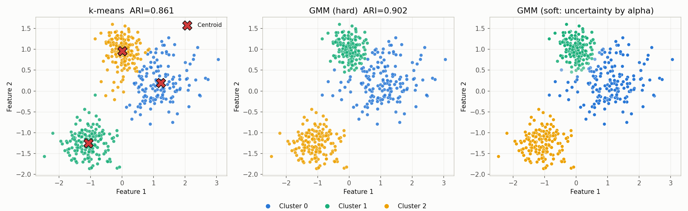
Running the code above produces the figure shown. From left to right: k-means, GMM (hard assignment), and GMM (soft assignment, where points closer to a cluster boundary are drawn with higher transparency). The fading colors near cluster boundaries visually confirm that GMM retains probabilistic membership rather than a simple majority vote.
Comparing agreement with the true cluster labels via sklearn.metrics.adjusted_rand_score (ARI, closer to 1 means better agreement), k-means scores 0.861 and GMM scores 0.902. Since this example uses clusters with different standard deviations (0.8/1.2/0.6), producing near-elliptical rather than spherical distributions, this quantitatively confirms that GMM, which can estimate a separate covariance matrix per cluster, captures the true structure more accurately than k-means, which assumes spherical clusters.
Edge Cases and Practical Pitfalls
Singular Covariance Matrices and Diverging Likelihood
The GMM log-likelihood harbors a serious pathology that textbooks rarely emphasize. If the (responsibility-weighted) data points assigned to a cluster \(j\) effectively number just one, or if multiple points are linearly dependent (collinear, or exact duplicates), the covariance matrix
\[ \boldsymbol{\Sigma}_j = \frac{\sum_i \gamma_{ij}(\mathbf{x}_i-\boldsymbol{\mu}_j)(\mathbf{x}_i-\boldsymbol{\mu}_j)^T}{\sum_i \gamma_{ij}} \]approaches a singular matrix (zero determinant, no inverse). Since the Gaussian density \(\mathcal{N}(\mathbf{x}|\boldsymbol{\mu},\boldsymbol{\Sigma}) \propto |\boldsymbol{\Sigma}|^{-1/2}\exp(\cdots)\) diverges as \(|\boldsymbol{\Sigma}| \to 0\) , the global supremum of the GMM log-likelihood is actually \(+\infty\) , achieved by a degenerate solution where one component collapses onto a single data point. This is a well-known pathology inherent to GMM’s maximum likelihood estimation (Day, 1969; McLachlan & Peel, 2000): if an EM iteration happens to drift toward such an assignment, the covariance approaches singularity, causing numerical instability or outright failure in later iterations.
The standard practical remedy is to regularize the covariance matrix by adding a small positive value to its diagonal (sklearn.mixture.GaussianMixture’s reg_covar parameter, default \(10^{-6}\)
), using \(\boldsymbol{\Sigma}_j + \text{reg\_covar}\cdot I\)
so the determinant never hits exactly zero.
Numerical verification: To reproduce this pathology, we built a dataset consisting of a main cluster of 200 normally distributed points plus 5 exact duplicate points at the identical coordinate \((10,10)\)
, and fit a 3-component GMM with reg_covar=0 (no regularization). scikit-learn actually raised an exception:
ValueError: Fitting the mixture model failed because some components have
ill-defined empirical covariance (for instance caused by singleton or
collapsed samples). Try to decrease the number of components, increase
reg_covar, or scale the input data.
This error occurs exactly as the theory predicts: one component tried to collapse onto the duplicate points, driving its covariance to singularity. Fitting the same data with the default reg_covar=1e-6 instead converges normally (total log-likelihood \(-524.729\)
), and the determinant of the covariance for the component that captured the duplicate points was \(1.0\times 10^{-12}\)
(versus \(0.496\)
and \(0.597\)
for the other two components) — more than eight orders of magnitude smaller. This component’s mixing weight was \(0.0244\)
, which matches exactly the number of duplicate points divided by the total sample count (\(5/205=0.0244\)
), quantitatively confirming that GMM was assigning one component almost entirely to these 5 points, approaching a degenerate solution. Without regularization, this component’s covariance would have continued shrinking, and the likelihood would in theory have diverged to infinity.
Local Optima and Initialization Dependence
The local-optima problem for k-means and its mitigation via k-means++ were discussed above (see “k-means++ and the Local Optima Problem”). There is a practical pitfall here that is easy to overlook. scikit-learn’s KMeans defaults n_init to 'auto', but this resolves to running only a single initialization when init='k-means++' (the default) — it resolves to 10 only when init='random' (confirmed in the implementation of sklearn.cluster._kmeans._BaseKMeans._check_params_vs_input). In other words, the assumption that “k-means++ automatically tries multiple times” is wrong: unless n_init is set explicitly, scikit-learn runs k-means++ initialization only once. The Python implementation example in this article (below) explicitly sets n_init=10, a deliberate choice given the local-optima risk we measured earlier (7 of 200 random-init runs, 3.5%, landed in a local optimum exceeding 1.5x the global optimum, versus 0 for k-means++).
GMM’s GaussianMixture likewise guarantees convergence only to a local maximum of the log-likelihood, and its n_init defaults explicitly to 1. Unlike KMeans, there is no clever 'auto' resolution logic, so when the cluster structure is complex, n_init should be increased explicitly.
Cluster Number Selection
Both k-means and GMM require specifying the number of clusters \(k\) in advance. We cover three standard selection criteria below, along with their theoretical basis and limitations.
Elbow Method
k-means’s inertia \(J\) decreases monotonically as \(k\) increases (reaching \(J=0\) at \(k=n\) ). The elbow method judges, by eye, the point where the decrease in inertia starts to flatten out — the “elbow.” There is no theoretical optimality guarantee; it is purely an empirical heuristic. When the decrease curve is smooth and the elbow is not clearly defined (as in the experiment below, e.g. when clusters are close together), the judgment becomes difficult, and it is best used together with silhouette analysis or BIC.
inertias = []
K_range = range(1, 10)
for k in K_range:
    km = KMeans(n_clusters=k, n_init=10, random_state=42)
    km.fit(X)
    inertias.append(km.inertia_)

plt.plot(K_range, inertias, 'bo-')
plt.xlabel('k')
plt.ylabel('Inertia')
plt.title('Elbow Method')
plt.grid(True, alpha=0.3)
plt.show()
Silhouette Score
\[s(i) = \frac{b(i) - a(i)}{\max(a(i), b(i))} \tag{8}\]where \(a(i)\) is the mean intra-cluster distance and \(b(i)\) is the mean nearest-cluster distance. \(s(i) \in [-1, 1]\) ; closer to 1 indicates better clustering.
A pitfall of silhouette analysis: The silhouette score selects the \(k\) that maximizes the tradeoff between intra-cluster cohesion and inter-cluster separation, but this does not necessarily coincide with the true number of clusters. In particular, when clusters are close together, merging two adjacent clusters into one can appear to improve inter-cluster separation, causing the silhouette score to favor a smaller \(k\) .
BIC (for GMM)
BIC (Bayesian Information Criterion) is derived by approximating the model evidence (marginal likelihood) \(p(D|k) = \int p(D|\theta,k)p(\theta|k)\,d\theta\) . Since this integral is intractable in high dimensions, we apply a Laplace approximation (a second-order Taylor expansion of the log-evidence, giving a Gaussian approximation) around the MLE \(\hat\theta\) :
\[ \log p(D|k) \approx \ell(\hat\theta) - \frac{1}{2}\log|\mathbf{H}| + \frac{p}{2}\log(2\pi) \]where \(p\) is the number of free parameters in the model and \(\mathbf{H}\) is the Hessian of the negative log-likelihood (the observed Fisher information matrix). For i.i.d. data, \(\mathbf{H} \approx n\bar{\mathbf{H}}\) (where \(\bar{\mathbf{H}}\) does not depend on the sample size), so \(\log|\mathbf{H}| \approx p\log n + \log|\bar{\mathbf{H}}|\) . As \(n\to\infty\) , only the \(p\log n\) term dominates, so dropping the constant terms that don’t depend on \(n\) gives
\[ \log p(D|k) \approx \ell(\hat\theta) - \frac{p}{2}\log n \](Schwarz, 1978). Multiplying by \(-2\) to turn this into a minimization problem gives the conventional definition of BIC:
\[ \text{BIC} = -2\,\ell(\hat\theta) + p\log n \]For a GMM with full covariance, the number of free parameters \(p\) consists of \(k-1\) mixing weights (only \(k-1\) are independent due to the constraint \(\sum_j\pi_j=1\) ), \(kd\) mean parameters, and \(k\) symmetric covariance matrices with \(d(d+1)/2\) entries each:
\[ p = (k-1) + kd + k\,\frac{d(d+1)}{2} \]AIC (Akaike Information Criterion) uses the same log-likelihood term but a penalty of \(2p\) instead (\(\text{AIC} = -2\ell(\hat\theta) + 2p\) ). Since BIC’s penalty \(p\log n\) grows with \(n\) , BIC penalizes model complexity more heavily than AIC as \(n\) grows, and so BIC tends to select a smaller \(k\) in general.
bics = []
K_range = range(1, 10)
for k in K_range:
    gm = GaussianMixture(n_components=k, random_state=42)
    gm.fit(X)
    bics.append(gm.bic(X))

plt.plot(K_range, bics, 'ro-')
plt.xlabel('k')
plt.ylabel('BIC')
plt.title('BIC for GMM')
plt.grid(True, alpha=0.3)
plt.show()
Select \(k\) that minimizes BIC.
Numerical Verification: Comparing Elbow, Silhouette, BIC, and AIC
For the same 3-cluster dataset used in the Python implementation above (true \(k=3\)
), we computed inertia, silhouette score, BIC, and AIC for \(k=2\)
through \(9\)
, and also checked that the number of free parameters computed from the formula for \(d=2,\,k=3\)
(\(p=(3-1)+3\cdot2+3\cdot3=17\)
) matches the value returned by GaussianMixture(n_components=3)._n_parameters().
| \(k\) | Inertia | Silhouette | BIC | AIC |
|---|---|---|---|---|
| 2 | 317.939 | 0.6331 | 2097.19 | 2050.83 |
| 3 | 147.347 | 0.6121 | 1928.32 | 1856.67 |
| 4 | 117.719 | 0.5667 | 1961.15 | 1864.21 |
| 5 | 100.437 | 0.4411 | 1981.18 | 1858.96 |
| 6 | 85.619 | 0.4339 | 2011.85 | 1864.34 |
| 7 | 73.735 | 0.4289 | 2045.50 | 1872.70 |
| 8 | 66.362 | 0.3417 | 2071.98 | 1873.89 |
| 9 | 58.198 | 0.3530 | 2106.07 | 1882.70 |
The number of free parameters matched the formula’s value of \(p=17\)
exactly, agreeing with _n_parameters(). The silhouette score was maximized at \(k=2\)
(score \(0.6331\)
), which does not match the true \(k=3\)
. This dataset has two of its three clusters generated close together (a cluster with std 1.2 adjacent to one with std 0.8), so merging them into 2 clusters apparently improved the perceived separation. BIC and AIC, on the other hand, both reached their minimum at \(k=3\)
(\(\text{BIC}=1928.32\)
, \(\text{AIC}=1856.67\)
), correctly identifying the true number of clusters. This empirically demonstrates that silhouette analysis should not be relied on as the sole criterion, and should be used together with density-based criteria like BIC/AIC and visual elbow-method inspection.
Related Articles
- Ensemble Learning: From Decision Trees to Random Forest and Gradient Boosting - Supervised learning methods; clustering results can serve as features.
- Understanding Self-Attention from Scratch: Math and Python Implementation - Similarity between Attention’s weighted averaging and GMM’s mixture model.
- Support Vector Machines (SVM): Kernel Methods and Nonlinear Classification with Python - Comparison with supervised classification; SVM finds boundaries while clustering discovers data structure.
- Markov Chain Monte Carlo (MCMC): Metropolis-Hastings and Gibbs Sampling - MCMC can also estimate GMM parameters.
- Bayesian Linear Regression: From Least Squares to Bayesian Estimation - Bayesian foundations underlying GMM.
- From SGD to Adam: Evolution of Gradient-Based Optimization - Understanding the relationship between EM and gradient methods.
- Machine Learning Hub for Time-Series, Classification, and Anomaly Detection - Hub article organizing k-means/GMM, ensembles, LSTM, and Kalman filters along 3 selection axes and 9 decision scenarios.
- Time-Series Anomaly Detection: From Statistical Methods to Kalman Filter in Python - Unsupervised anomaly detection extending clustering; low-density points or component responsibilities serve as anomaly scores.
References
- Bishop, C. M. (2006). Pattern Recognition and Machine Learning . Springer. Chapters 9.
- MacQueen, J. (1967). “Some methods for classification and analysis of multivariate observations”. Proceedings of the 5th Berkeley Symposium.
- scikit-learn Clustering documentation