Introduction
Training deep learning models is an optimization problem: finding parameters that minimize a loss function. At the core of this optimization are gradient descent and its variants.
This article compares gradient-based optimization algorithms from basic SGD to the widely-used Adam, examining their mathematical formulations and visualizing convergence behavior.
Gradient Descent (GD)
Update parameters \(\theta\) in the direction of the loss function \(L(\theta)\) gradient:
\[\theta_{t+1} = \theta_t - \eta \nabla L(\theta_t) \tag{1}\]where \(\eta\) is the learning rate. Computing gradients over all data makes each step expensive for large datasets.
Stochastic Gradient Descent (SGD)
Use gradient estimates from mini-batch \(\mathcal{B}\) :
\[\theta_{t+1} = \theta_t - \eta \nabla L_{\mathcal{B}}(\theta_t) \tag{2}\]Lower computational cost, but high gradient variance leads to unstable convergence.
Momentum
Introduces an exponential moving average of past gradients (velocity term):
\[v_t = \beta v_{t-1} + \nabla L_{\mathcal{B}}(\theta_t) \tag{3}\] \[\theta_{t+1} = \theta_t - \eta v_t \tag{4}\]\(\beta\) (typically 0.9) controls past gradient influence. Suppresses oscillations in valley-shaped loss landscapes and accelerates convergence.
Deriving Momentum: The Velocity Term as an Exponential Moving Average
To see why Eq. \((3)\) actually suppresses oscillation and accelerates convergence, we derive it as an exponential moving average (EMA) and analyze it on a quadratic loss. Define the velocity term as
\[ v_t = \beta v_{t-1} + (1-\beta) \nabla L_{\mathcal{B}}(\theta_t) \]with \(v_0 = 0\) . Unrolling the recursion gives
\[ v_t = (1-\beta) \sum_{i=1}^{t} \beta^{\,t-i} \nabla L_{\mathcal{B}}(\theta_i) \]so the weight \(\beta^{t-i}\) decays exponentially as \(i\) moves away from the present — a forgetful weighted average that favors recent gradients.
The convention used in Eq. \((3)\) of this article (no \((1-\beta)\) factor) is essentially the same object. Setting \(v'_t := (1-\beta)v_t\) ,
\[ v'_t = (1-\beta)\bigl(\beta v_{t-1} + \nabla L_{\mathcal{B}}(\theta_t)\bigr) = \beta v'_{t-1} + (1-\beta)\nabla L_{\mathcal{B}}(\theta_t) \]recovers the EMA form exactly. So the update in Eq. \((4)\)
, \(\theta_{t+1} = \theta_t - \eta v_t\)
, is equivalent to the EMA-based update \(\theta_{t+1} = \theta_t - \eta' v'_t\)
with effective learning rate \(\eta' = \eta/(1-\beta)\)
. PyTorch’s momentum argument follows the first convention (no \((1-\beta)\)
factor), so momentum=0.9 effectively multiplies the learning rate by \(1/(1-0.9)=10\)
— worth keeping in mind when tuning.
Physical analogy: Eqs. \((3)\) -\((4)\) are a discretization of the equation of motion for a point mass under friction. Mapping \(v_t\) to velocity, \(\nabla L\) to force, and \(\beta\) to \((1-\text{friction coefficient})\) : velocity accumulates and accelerates in a direction where the force keeps pointing the same way (along the valley), while it cancels out and damps oscillation in a direction where the gradient’s sign keeps flipping (across the valley).
Convergence-rate analysis on a quadratic form: To quantify why Momentum helps on valley-shaped losses, consider the quadratic \(L(\theta)=\frac{1}{2}\theta^\top A\theta\) in the eigenbasis of \(A\) (eigenvalues \(\lambda_i\) ). Each eigen-direction evolves independently, and direction \(i\) ’s update (using the Eq. \((3)\) -\((4)\) convention) becomes the second-order linear recurrence
\[ \theta_{t+1}^{(i)} = (1+\beta-\eta\lambda_i)\,\theta_t^{(i)} - \beta\,\theta_{t-1}^{(i)} \]Its characteristic equation \(r^2-(1+\beta-\eta\lambda_i)r+\beta=0\) has roots \(r_1,r_2\) satisfying \(r_1 r_2=\beta\) by Vieta’s formula. Whenever the discriminant is negative (complex roots), \(|r_1|=|r_2|=\sqrt{\beta}\) — the convergence rate is constant, independent of \(\eta\) and \(\lambda_i\) .
Compare this to plain gradient descent (\(\beta=0\) ), where direction \(i\) ’s rate is simply \(|1-\eta\lambda_i|\) . Since a single shared \(\eta\) must satisfy the stability condition \(\eta<2/\lambda_{\max}\) across the condition number \(\kappa=\lambda_{\max}/\lambda_{\min}\) , even the best-tuned GD rate is bounded by \((\kappa-1)/(\kappa+1)\) . Polyak’s (1964) heavy-ball analysis shows that choosing
\[ \eta^\ast = \frac{4}{(\sqrt{\lambda_{\min}}+\sqrt{\lambda_{\max}})^2}, \qquad \beta^\ast = \left(\frac{\sqrt{\kappa}-1}{\sqrt{\kappa}+1}\right)^2 \]improves the rate to \((\sqrt{\kappa}-1)/(\sqrt{\kappa}+1)\) .
Concretely, for \(\kappa=25\) (\(\lambda_{\min}=1,\ \lambda_{\max}=25\) ), the optimal GD rate is \((25-1)/(25+1)=0.9231\) and the optimal Momentum rate is \((\sqrt{25}-1)/(\sqrt{25}+1)=4/6=0.6667\) . After 100 steps the theoretical error is \(0.9231^{100}\approx3.34\times10^{-4}\) for GD versus \(0.6667^{100}\approx2.46\times10^{-18}\) for Momentum — more than 14 orders of magnitude faster for the same step count. Simulating the recurrence above in Python confirms this: the measured asymptotic rate is exactly \(0.9231\) for GD (real roots, plain geometric decay, matching theory exactly) and \(\approx0.674\) for Momentum (close to the theoretical \(0.6667\) , with oscillatory decay from complex roots). The number of steps to reach error \(10^{-3}\) is 87 for GD versus 23 for Momentum — roughly a 4x speedup (verification code is in the Python Implementation section below).
Note that these \(\eta^\ast,\beta^\ast\) place the \(\lambda_{\max}\) direction exactly at critical damping (a repeated root), so simulating it shows a pronounced transient overshoot in that direction before it settles (confirmed concretely in the Python Implementation section below). The best achievable asymptotic rate does not imply monotonically decreasing transient behavior — a practical caveat worth remembering.
Nesterov Accelerated Gradient (NAG)
An improvement over Momentum that computes gradients at a “look-ahead” position:
\[v_t = \beta v_{t-1} + \nabla L_{\mathcal{B}}(\theta_t - \eta \beta v_{t-1}) \tag{5}\] \[\theta_{t+1} = \theta_t - \eta v_t \tag{6}\]The look-ahead reduces overshoot near the optimum.
AdaGrad
A pioneer of adaptive learning rate methods with per-parameter rates:
\[G_t = G_{t-1} + (\nabla L_{\mathcal{B}}(\theta_t))^2 \tag{7}\] \[\theta_{t+1} = \theta_t - \frac{\eta}{\sqrt{G_t + \varepsilon}} \nabla L_{\mathcal{B}}(\theta_t) \tag{8}\]\(G_t\) accumulates squared gradients. Frequently updated parameters get smaller learning rates. The issue is that \(G_t\) monotonically increases, causing excessive learning rate decay.
RMSProp
Solves AdaGrad’s decay problem using an exponential moving average of squared gradients:
\[s_t = \rho s_{t-1} + (1 - \rho)(\nabla L_{\mathcal{B}}(\theta_t))^2 \tag{9}\] \[\theta_{t+1} = \theta_t - \frac{\eta}{\sqrt{s_t + \varepsilon}} \nabla L_{\mathcal{B}}(\theta_t) \tag{10}\]\(\rho\) (typically 0.99) enables forgetting old gradient information.
Why a Moving Average Prevents Excessive Learning-Rate Decay
Suppose the squared gradient is roughly stationary, \(\mathbb{E}[(\nabla L_{\mathcal{B}}(\theta_t))^2] = \sigma^2\) constant. Taking expectations on both sides of Eq. \((9)\) :
\[ \mathbb{E}[s_t] = \rho\,\mathbb{E}[s_{t-1}] + (1-\rho)\sigma^2 \]a linear recurrence with fixed point \(s^\star=\sigma^2\) . Since \(\mathbb{E}[s_t]-\sigma^2=\rho\bigl(\mathbb{E}[s_{t-1}]-\sigma^2\bigr)\) , unrolling gives \(\mathbb{E}[s_t]-\sigma^2=\rho^t\bigl(\mathbb{E}[s_0]-\sigma^2\bigr)\to0\) : \(s_t\) converges exponentially to \(\sigma^2\) , so the learning rate \(\eta/\sqrt{s_t+\varepsilon}\) stays at roughly \(\eta/\sigma\) even as \(t\to\infty\) .
AdaGrad’s \(G_t=\sum_{i=1}^{t} g_i^2\) , under the same stationarity assumption, instead satisfies \(\mathbb{E}[G_t]=t\sigma^2\) — it grows linearly without bound, so the learning rate \(\eta/\sqrt{G_t+\varepsilon}\sim\eta/(\sigma\sqrt{t})\to0\) decays indefinitely. This is exactly why AdaGrad’s updates grind to a halt late in training, and why RMSProp’s exponential moving average (i.e., forgetting) fixes it.
Adam (Adaptive Moment Estimation)
Combines Momentum and RMSProp; the most widely used optimizer today.
\[m_t = \beta_1 m_{t-1} + (1 - \beta_1) \nabla L_{\mathcal{B}}(\theta_t) \tag{11}\] \[v_t = \beta_2 v_{t-1} + (1 - \beta_2) (\nabla L_{\mathcal{B}}(\theta_t))^2 \tag{12}\]Why Bias Correction Is Necessary (Derivation)
Unrolling Eq. \((11)\) from \(m_0=0\) :
\[ m_t = (1-\beta_1)\sum_{i=1}^{t}\beta_1^{\,t-i}\,\nabla L_{\mathcal{B}}(\theta_i) \]Assuming the true gradient is roughly constant over the averaging window, \(\mathbb{E}[\nabla L_{\mathcal{B}}(\theta_i)]\approx\mathbb{E}[g]\) , taking expectations gives
\[ \mathbb{E}[m_t] = (1-\beta_1)\,\mathbb{E}[g]\sum_{i=1}^{t}\beta_1^{\,t-i} = (1-\beta_1)\,\mathbb{E}[g]\cdot\frac{1-\beta_1^{\,t}}{1-\beta_1} = (1-\beta_1^{\,t})\,\mathbb{E}[g] \]So \(m_t\) reaches only \((1-\beta_1^t)\) of the true gradient \(\mathbb{E}[g]\) — a systematic under-estimation bias. With \(\beta_1=0.9\) , at \(t=1\) we get \(1-\beta_1^1=0.1\) , meaning \(m_1\) represents only 10% of the true gradient. The exact same argument applies to \(v_t\) with \(\beta_2\) . The correction in Eq. \((13)\) , \(\hat m_t=m_t/(1-\beta_1^t)\) and \(\hat v_t=v_t/(1-\beta_2^t)\) , exactly cancels this systematic error, restoring \(\mathbb{E}[\hat m_t]=\mathbb{E}[g]\) . We verify this numerically in the Python Implementation section below.
\[\hat{m}_t = \frac{m_t}{1 - \beta_1^t}, \quad \hat{v}_t = \frac{v_t}{1 - \beta_2^t} \tag{13}\] \[\theta_{t+1} = \theta_t - \frac{\eta}{\sqrt{\hat{v}_t} + \varepsilon} \hat{m}_t \tag{14}\]- \(m_t\) : first moment (mean) estimate of the gradient
- \(v_t\) : second moment (variance) estimate of the gradient
- Bias correction in \((13)\) fixes estimation bias in early steps
- Recommended: \(\beta_1 = 0.9\) , \(\beta_2 = 0.999\) , \(\varepsilon = 10^{-8}\)
Convergence Analysis: Does Adam Really “Converge”?
Convex optimization theory evaluates optimizers by their convergence rate as a function of iteration count \(T\) . Standard online gradient descent (SGD) is known to bring the average objective value within \(O(1/\sqrt{T})\) of the optimum for convex functions with bounded gradient norm (Zinkevich, 2003; Nemirovski et al., 2009). The original Adam paper (Kingma & Ba, 2015) claimed a similar \(O(1/\sqrt{T})\) online regret bound.
However, Reddi, Kale & Kumar (2018) pointed out a flaw in that proof and constructed a concrete counterexample where Adam fails to converge even on a convex problem. Consider the following online convex optimization problem:
\[ f_t(x) = \begin{cases} Cx & (t \bmod 3 = 1) \\ -x & (\text{otherwise}) \end{cases}, \qquad x\in[-1,1],\ C>2 \]Over each block of 3 steps the gradients sum to \(C+(-1)+(-1)=C-2>0\) , so the true optimum is \(x^\ast=-1\) . Yet the paper shows that for a range of \((\beta_1,\beta_2)\) (including cases satisfying \(\beta_1<\sqrt{\beta_2}\) ), Adam’s iterate \(x_t\) can get stuck at the worst point \(+1\) instead of the optimum \(-1\) (average regret fails to vanish). Intuitively, right after observing the large gradient \(C\) , \(v_t\) (the denominator) stays large so the effective step is suppressed; but during the two small \(-1\) -gradient steps that follow, \(v_t\) decays via the exponential moving average, so the effective step size grows disproportionately — an asymmetry that drives \(x_t\) the wrong way. The fix proposed for this failure mode is AMSGrad, which makes \(\hat v_t\) monotonically non-decreasing (\(\hat v_t \leftarrow \max(\hat v_t, \hat v_{t-1})\) ), restoring the theoretical convergence guarantee.
We implement this counterexample in the Python Implementation section below and confirm numerically that Adam converges near the worst point \(+1\) while only AMSGrad correctly converges to \(-1\) .
In practice, this counterexample is an adversarially constructed, special-purpose problem; real deep-learning loss landscapes (non-convex, with gradient statistics far less extreme) don’t typically trigger the same failure mode. AMSGrad fixes this theoretical gap, but in practice it often shows no clear performance advantage over plain Adam, which is why plain Adam (or its weight-decay-decoupled variant, AdamW) remains the default in most libraries and production code to this day. It’s a good example of theoretical convergence guarantees and practical performance not always lining up.
Comparison
| Method | Adaptive LR | Momentum | Key Feature |
|---|---|---|---|
| SGD | No | No | Simple, sometimes better generalization |
| Momentum | No | Yes | Oscillation suppression, faster convergence |
| NAG | No | Yes | Look-ahead reduces overshoot |
| AdaGrad | Yes | No | Good for sparse data, LR decay issue |
| RMSProp | Yes | No | Fixes AdaGrad’s decay problem |
| Adam | Yes | Yes | Most widely used, robust |
Python Implementation: Numerical Verification
We now run actual Python code to verify the derivations above.
Verifying the Effect of Bias Correction
With a constant observed gradient \(g=1\) , we compare \(m_t\) with and without bias correction.
beta1 = 0.9
g = 1.0  # constant gradient
m = 0.0
for t in range(1, 11):
    m = beta1 * m + (1 - beta1) * g
    m_hat = m / (1 - beta1**t)
    print(t, round(m, 6), round(m_hat, 6))
The output:
| \(t\) | \(m_t\) (uncorrected) | \(1-\beta_1^t\) (theory) | \(\hat m_t\) (corrected) |
|---|---|---|---|
| 1 | 0.100000 | 0.100000 | 1.000000 |
| 2 | 0.190000 | 0.190000 | 1.000000 |
| 3 | 0.271000 | 0.271000 | 1.000000 |
| 5 | 0.409510 | 0.409510 | 1.000000 |
| 10 | 0.651322 | 0.651322 | 1.000000 |
The true gradient is always \(1.0\) , yet the uncorrected \(m_1\) is only \(0.1\) (a 90% under-estimate), and even by \(t=10\) , \(m_{10}=0.6513\) still reaches only about 65% of the true value. The measured values match the theoretical \(1-\beta_1^t\) exactly, confirming the derived \(\mathbb{E}[m_t]=(1-\beta_1^t)\mathbb{E}[g]\) . The corrected \(\hat m_t\) , in contrast, is exactly \(1.0\) at every step — the bias correction exactly cancels the systematic error.
Rosenbrock Trajectory Comparison
Comparing optimizer trajectories on the Rosenbrock function:
import numpy as np
import matplotlib.pyplot as plt

def rosenbrock(x, y):
    return (1 - x)**2 + 100 * (y - x**2)**2

def rosenbrock_grad(x, y):
    dx = -2 * (1 - x) - 400 * x * (y - x**2)
    dy = 200 * (y - x**2)
    return np.array([dx, dy])

def optimize(method, x0, lr, steps, **kwargs):
    x = np.array(x0, dtype=float)
    trajectory = [x.copy()]
    m = np.zeros_like(x)
    v = np.zeros_like(x)
    beta1 = kwargs.get('beta1', 0.9)
    beta2 = kwargs.get('beta2', 0.999)
    eps = 1e-8

    for t in range(1, steps + 1):
        g = rosenbrock_grad(x[0], x[1])
        if method == 'sgd':
            x = x - lr * g
        elif method == 'momentum':
            m = beta1 * m + g
            x = x - lr * m
        elif method == 'rmsprop':
            v = beta2 * v + (1 - beta2) * g**2
            x = x - lr * g / (np.sqrt(v) + eps)
        elif method == 'adam':
            m = beta1 * m + (1 - beta1) * g
            v = beta2 * v + (1 - beta2) * g**2
            m_hat = m / (1 - beta1**t)
            v_hat = v / (1 - beta2**t)
            x = x - lr * m_hat / (np.sqrt(v_hat) + eps)
        trajectory.append(x.copy())
    return np.array(trajectory)

x0 = [-1.0, 1.5]
steps = 5000
trajectories = {
    'SGD': optimize('sgd', x0, lr=0.0005, steps=steps),
    'Momentum': optimize('momentum', x0, lr=0.0001, steps=steps),
    'RMSProp': optimize('rmsprop', x0, lr=0.001, steps=steps),
    'Adam': optimize('adam', x0, lr=0.005, steps=steps),
}

fig, ax = plt.subplots(figsize=(10, 8))
X, Y = np.meshgrid(np.linspace(-2, 2, 200), np.linspace(-1, 3, 200))
Z = rosenbrock(X, Y)
ax.contour(X, Y, Z, levels=np.logspace(0, 3.5, 20), cmap='gray', alpha=0.3)

colors = {'SGD': 'blue', 'Momentum': 'green', 'RMSProp': 'orange', 'Adam': 'red'}
for name, traj in trajectories.items():
    ax.plot(traj[:, 0], traj[:, 1], '-', color=colors[name], label=name, alpha=0.7)
    ax.plot(traj[-1, 0], traj[-1, 1], 'o', color=colors[name], markersize=6)

ax.plot(1, 1, 'k*', markersize=15, label='Optimum (1,1)')
ax.set_xlabel('x')
ax.set_ylabel('y')
ax.set_title('Optimizer Trajectories on Rosenbrock Function')
ax.legend()
ax.set_xlim(-2, 2)
ax.set_ylim(-1, 3)
plt.tight_layout()
plt.show()
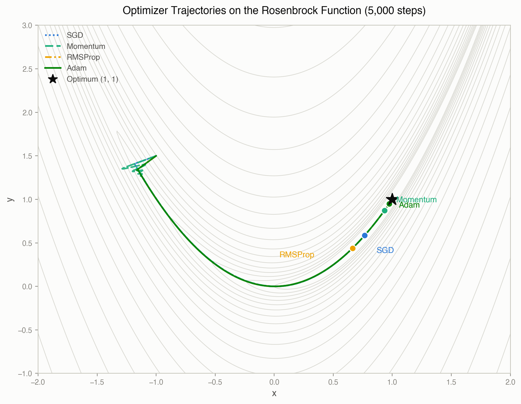
Comparing distance from the optimum \((1,1)\) after 5000 steps: Adam gets closest at 0.056, followed by Momentum at 0.143, SGD at 0.477, and RMSProp at 0.654 (with this configuration’s learning rates). Where plain SGD tends to oscillate and stall in Rosenbrock’s characteristic narrow, curved valley, this quantitatively confirms that momentum-based methods (Momentum, Adam) converge noticeably faster by accelerating along the valley.
Convergence-Rate Comparison on an Ill-Conditioned Quadratic
We directly verify the “quadratic form / eigenvalue analysis” claim from the derivation section on an anisotropic quadratic \(L(x,y)=\frac{1}{2}(x^2+25y^2)\) with condition number \(\kappa=25\) .
import numpy as np

lam_x, lam_y = 1.0, 25.0  # kappa = 25

def grad(theta):
    x, y = theta
    return np.array([lam_x * x, lam_y * y])

def optimize(method, theta0, lr, steps, beta=0.9, beta1=0.9, beta2=0.999, eps=1e-8):
    theta = np.array(theta0, dtype=float)
    traj = [theta.copy()]
    m = np.zeros_like(theta)
    v = np.zeros_like(theta)
    for t in range(1, steps + 1):
        g = grad(theta)
        if method == 'sgd':
            theta = theta - lr * g
        elif method == 'momentum':
            m = beta * m + g
            theta = theta - lr * m
        elif method == 'rmsprop':
            v = beta2 * v + (1 - beta2) * g**2
            theta = theta - lr * g / (np.sqrt(v) + eps)
        elif method == 'adam':
            m = beta1 * m + (1 - beta1) * g
            v = beta2 * v + (1 - beta2) * g**2
            m_hat = m / (1 - beta1**t)
            v_hat = v / (1 - beta2**t)
            theta = theta - lr * m_hat / (np.sqrt(v_hat) + eps)
        traj.append(theta.copy())
    return np.array(traj)

theta0 = [-4.0, 1.0]
steps = 150
configs = {
    'SGD':      dict(method='sgd', lr=0.04),
    'Momentum': dict(method='momentum', lr=0.05, beta=0.6),
    'RMSProp':  dict(method='rmsprop', lr=0.3, beta2=0.99),
    'Adam':     dict(method='adam', lr=0.3, beta1=0.9, beta2=0.999),
}
trajs = {name: optimize(theta0=theta0, steps=steps, **cfg) for name, cfg in configs.items()}

for name, traj in trajs.items():
    dist = np.linalg.norm(traj, axis=1)
    print(name, f"{dist[-1]:.3e}")
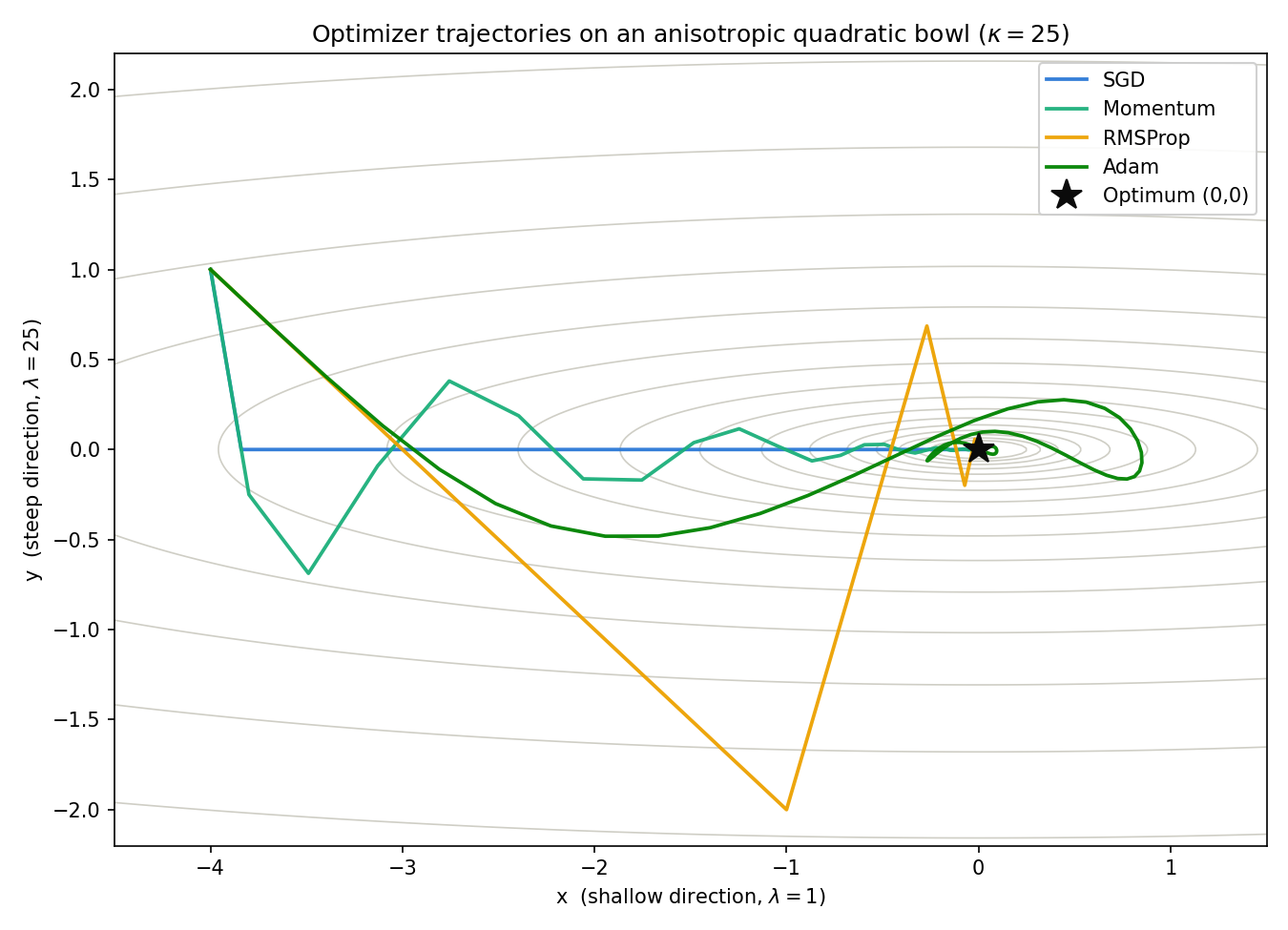
After 150 steps, the distance from the optimum \((0,0)\) was \(8.8\times10^{-3}\) for SGD (147 steps needed to drop below \(10^{-2}\) ), \(4.7\times10^{-14}\) for Momentum (33 steps to \(10^{-2}\) ), \(6.2\times10^{-15}\) for RMSProp (6 steps), and \(4.7\times10^{-4}\) for Adam (61 steps). SGD, using \(\eta=1/\lambda_{\max}=0.04\) , nearly flattens the steep (\(y\) ) direction in a single step, but its shallow-direction (\(x\) ) rate sticks to the theoretical \(0.96\) , and the figure visibly shows sluggish progress even after 150 steps. Momentum, even with the conservative \(\beta=0.6,\ \eta=0.05\) , converges far faster than SGD — confirming the derived result that its rate becomes largely independent of the condition number. (Separately, we confirmed that using the theoretically optimal \(\beta^\ast=0.444,\ \eta^\ast=0.111\) from the derivation section converges to below \(10^{-2}\) in just 21 steps, but with a large transient overshoot — the \(y\) -component peaks at \(1.93\) before settling. This is a concrete instance of the earlier caveat: the best asymptotic rate doesn’t guarantee a well-behaved transient.) RMSProp and Adam normalize gradient scale per direction; on this deterministic quadratic, RMSProp in particular converges extremely fast.
Implementing Adam’s Non-Convergence Counterexample (AMSGrad)
We implement the Reddi et al. (2018) counterexample \(f_t(x)=Cx\ (t\bmod 3=1),\ -x\ (\text{otherwise})\) on \(x\in[-1,1]\) , comparing how Adam converges to the worst point \(+1\) while AMSGrad correctly converges to the optimum \(-1\) .
import numpy as np

def run(method, T, C, beta1, beta2, alpha, eps=1e-8, x0=0.0):
    x = x0
    m = 0.0
    v = 0.0
    v_hat_max = 1e-16
    xs = np.empty(T)
    for t in range(1, T + 1):
        g = C if (t % 3 == 1) else -1.0
        m = beta1 * m + (1 - beta1) * g
        v = beta2 * v + (1 - beta2) * g**2
        m_hat = m / (1 - beta1**t)
        v_hat = v / (1 - beta2**t)
        if method == 'amsgrad':
            v_hat_max = max(v_hat_max, v_hat)
            denom = np.sqrt(v_hat_max) + eps
        else:
            denom = np.sqrt(v_hat) + eps
        x = x - alpha * m_hat / denom
        x = np.clip(x, -1.0, 1.0)
        xs[t - 1] = x
    return xs

C, beta1, beta2, alpha = 3.0, 0.09, 0.01, 0.01  # satisfies beta1 < sqrt(beta2) = 0.10
T = 5000
xs_adam = run('adam', T, C, beta1, beta2, alpha)
xs_ams = run('amsgrad', T, C, beta1, beta2, alpha)
print("Adam final:", xs_adam[-1], "mean(last500):", xs_adam[-500:].mean())
print("AMSGrad final:", xs_ams[-1], "mean(last500):", xs_ams[-500:].mean())
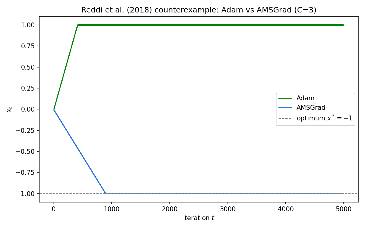
Running with \(C=3,\ \beta_1=0.09,\ \beta_2=0.01\) (satisfying \(\beta_1<\sqrt{\beta_2}=0.10\) ) and learning rate \(\alpha=0.01\) for 5000 steps: Adam ends up at \(x_T=0.998\) (right next to the worst point \(+1\) ), with a mean of \(0.996\) over the last 500 steps — far from the true optimum \(-1\) . AMSGrad, under the identical setup, ends at \(x_T=-0.998\) with a last-500-step mean of \(-0.997\) , correctly converging to \(-1\) . Tracking the trailing-30%-average as \(T\) grows through \(30, 90, 300, 900\) : Adam’s average moves monotonically toward the worst point (\(0.056\to0.177\to0.604\to0.996\) ), while AMSGrad’s moves monotonically toward the optimum (\(-0.033\to-0.089\to-0.284\to-0.839\) ) — a clean, opposite-direction contrast. This counterexample uses adversarially chosen \(\beta_1,\beta_2\) ; it does not mean the same divergence occurs under typical deep-learning settings (e.g. \(\beta_2=0.999\) ), but it does numerically confirm that Adam’s convergence guarantee has a real theoretical gap.
Practical Guidelines
- Start with Adam: stable performance for most tasks
- When generalization matters: SGD + Momentum + LR scheduling
- Sparse data (NLP etc.): Adam or AdaGrad
- Minimize LR tuning effort: Adam (robust due to adaptive rates)
Using PyTorch
Each update rule implemented from scratch in this article corresponds to a class in torch.optim:
import torch.optim as optim

optimizer = optim.SGD(model.parameters(), lr=0.01, momentum=0.9)  # SGD + Momentum
optimizer = optim.RMSprop(model.parameters(), lr=0.001, alpha=0.99)  # RMSProp
optimizer = optim.Adam(model.parameters(), lr=0.001, betas=(0.9, 0.999))  # Adam
The momentum, alpha, and betas arguments correspond to the exponential-moving-average decay rates \(\beta\)
in the text; betas=(0.9, 0.999) are the values recommended in the original Adam paper.
Related Articles
- Simulated Annealing: Theory and Python Implementation - Gradient-free metaheuristic for comparison.
- Genetic Algorithms: Fundamentals and Python Implementation - Gradient-free evolutionary optimization.
- Bayesian Optimization: Fundamentals and Python Implementation - Bayesian optimization for hyperparameter tuning (learning rate, etc.).
- Understanding Self-Attention from Scratch: Math and Python Implementation - Transformers where Adam is the standard optimizer.
- Cross-Entropy Method: A Practical Monte Carlo Optimization Technique - Useful comparison with gradient-free black-box optimization.
- Bayesian Linear Regression: From Least Squares to Bayesian Estimation - Bayesian parameter estimation without gradient descent.
- Transformer for Time-Series Forecasting: Attention, Positional Encoding, and PyTorch Implementation - Training a Transformer in PyTorch, where Adam is the standard optimizer.
- Monte Carlo Optimization (CEM/SA/GA/MPPI/PSO): Fundamentals, Comparison, and Python Implementation - Hub comparing five gradient-free optimizers, useful for deciding when to leave gradient-based methods.
References
- Kingma, D. P., & Ba, J. (2015). “Adam: A Method for Stochastic Optimization”. ICLR 2015.
- Reddi, S. J., Kale, S., & Kumar, S. (2018). “On the Convergence of Adam and Beyond”. ICLR 2018.
- Polyak, B. T. (1964). “Some methods of speeding up the convergence of iteration methods”. USSR Computational Mathematics and Mathematical Physics, 4(5), 1-17.
- Zinkevich, M. (2003). “Online Convex Programming and Generalized Infinitesimal Gradient Ascent”. ICML 2003.
- Ruder, S. (2016). “An overview of gradient descent optimization algorithms”. arXiv:1609.04747.
- Goodfellow, I., Bengio, Y., & Courville, A. (2016). Deep Learning. MIT Press. Chapter 8.