Introduction
Support Vector Machine (SVM) is a supervised learning method for classification and regression. It constructs a decision boundary that maximizes the margin between classes, achieving high generalization performance.
This article derives, without skipping steps, why the margin-maximization problem turns into a different optimization problem called the “dual problem,” and what the KKT conditions that appear along the way actually mean. The derivation is then cross-checked against the internal variables of a model trained with sklearn.svm.SVC, confirming numerically that theory and implementation agree. The mathematical validity of the kernel trick (Mercer’s theorem) and the infinite-dimensionality of the RBF kernel are covered in the follow-up article
SVM Kernel Design
; this article focuses on the foundational theory — margin maximization, dual derivation, and soft margin.
Linear SVM
Hard Margin
For linearly separable data \(\{(\mathbf{x}_i, y_i)\}_{i=1}^{n}\) (\(y_i \in \{-1, +1\}\) ), the decision boundary is found by solving:
\[\min_{\mathbf{w}, b} \frac{1}{2} \|\mathbf{w}\|^2 \tag{1}\] \[\text{subject to} \quad y_i(\mathbf{w} \cdot \mathbf{x}_i + b) \geq 1, \quad \forall i \tag{2}\]The signed distance from a point \(\mathbf{x}_i\) to the hyperplane \(\mathbf{w}\cdot\mathbf{x}+b=0\) is \((\mathbf{w}\cdot\mathbf{x}_i+b)/\|\mathbf{w}\|\) . Constraint (2) forces this distance to be at least \(1/\|\mathbf{w}\|\) in absolute value, so the total margin width across both classes is \(2/\|\mathbf{w}\|\) . Minimizing \(\|\mathbf{w}\|\) is therefore equivalent to maximizing the margin, and (1)-(2) is exactly “find the hyperplane that maximizes the margin,” written as a convex quadratic program.
Soft Margin
For non-separable data, introduce slack variables \(\xi_i \geq 0\) :
\[\min_{\mathbf{w}, b, \xi} \frac{1}{2} \|\mathbf{w}\|^2 + C \sum_{i=1}^{n} \xi_i \tag{3}\] \[\text{subject to} \quad y_i(\mathbf{w} \cdot \mathbf{x}_i + b) \geq 1 - \xi_i, \quad \xi_i \geq 0 \tag{4}\]\(C\) controls the trade-off between margin size and misclassification penalty. The value of \(\xi_i\) describes each sample’s state:
- \(\xi_i = 0\) : correctly classified, outside the margin
- \(0 < \xi_i \leq 1\) : correctly classified, but inside the margin
- \(\xi_i > 1\) : misclassified
The hard margin (1)-(2) is the limit of the soft margin as \(C \to \infty\) (no misclassification tolerated at all). The dual derivation below is carried out for the general soft-margin case, of which the hard margin is a special case.
Deriving the Lagrangian Dual and the KKT Conditions
The Lagrangian
For the inequality constraints of the primal (3)-(4), introduce a multiplier \(\alpha_i \geq 0\) for the margin constraint \(y_i(\mathbf{w}\cdot\mathbf{x}_i+b) - 1 + \xi_i \geq 0\) , and a multiplier \(\mu_i \geq 0\) for the non-negativity constraint \(\xi_i \geq 0\) . This gives the Lagrangian:
\[ L(\mathbf{w}, b, \xi, \alpha, \mu) = \frac{1}{2}\|\mathbf{w}\|^2 + C\sum_{i=1}^{n}\xi_i - \sum_{i=1}^{n}\alpha_i\big[y_i(\mathbf{w}\cdot\mathbf{x}_i+b) - 1 + \xi_i\big] - \sum_{i=1}^{n}\mu_i\xi_i \tag{5} \]The primal is equivalent to \(\min_{\mathbf{w},b,\xi}\max_{\alpha\geq 0,\mu\geq 0} L\) . The dual problem swaps the order to \(\max\min\) ; it is obtained by solving the inner minimization \(\min_{\mathbf{w},b,\xi} L\) analytically.
Stationarity (the first part of the KKT conditions)
Differentiate \(L\) with respect to \(\mathbf{w}, b, \xi_i\) and set to zero (the first-order condition of the inner minimization):
\[ \frac{\partial L}{\partial \mathbf{w}} = \mathbf{w} - \sum_{i=1}^{n}\alpha_i y_i \mathbf{x}_i = 0 \quad\Longrightarrow\quad \mathbf{w} = \sum_{i=1}^{n}\alpha_i y_i \mathbf{x}_i \tag{6} \] \[ \frac{\partial L}{\partial b} = -\sum_{i=1}^{n}\alpha_i y_i = 0 \quad\Longrightarrow\quad \sum_{i=1}^{n}\alpha_i y_i = 0 \tag{7} \] \[ \frac{\partial L}{\partial \xi_i} = C - \alpha_i - \mu_i = 0 \quad\Longrightarrow\quad \mu_i = C - \alpha_i \tag{8} \]Equation (6) says the normal vector \(\mathbf{w}\) of the decision boundary can be written as a weighted sum of the training data; (7) is an equality constraint on the dual variables; and (8), combined with \(\mu_i \geq 0\) , gives the upper bound \(\alpha_i \leq C\) .
Summary of the KKT Conditions
The stationarity conditions (6)-(8), together with the following, constitute the Karush-Kuhn-Tucker (KKT) conditions:
- Primal feasibility: \(y_i(\mathbf{w}\cdot\mathbf{x}_i+b) - 1 + \xi_i \geq 0\) , \(\xi_i \geq 0\)
- Dual feasibility: \(\alpha_i \geq 0\) , \(\mu_i \geq 0\) (combined with (8), this gives \(0 \leq \alpha_i \leq C\) )
- Complementary slackness: \( \alpha_i\big[y_i(\mathbf{w}\cdot\mathbf{x}_i+b) - 1 + \xi_i\big] = 0, \qquad \mu_i\xi_i = 0 \tag{9} \)
Because the primal is a convex quadratic program (convex objective, affine constraints), the KKT conditions are necessary and sufficient for global optimality. Complementary slackness (9) means: if a constraint holds with slack (strict inequality), its multiplier must be zero; if a multiplier is positive, the corresponding constraint must hold with equality. This is exactly what underlies the classification of support vectors in the next section.
Substituting Back to Obtain the Dual
Substitute (6)-(8) into (5) to eliminate \(\mathbf{w}, b, \xi\) . The terms containing \(\xi_i\) become
\[ C\xi_i - \alpha_i\xi_i - \mu_i\xi_i = \xi_i(C - \alpha_i - \mu_i) = 0 \quad (\text{by (8)}) \]and vanish entirely; the term containing \(b\) vanishes via (7) as \(-b\sum_i \alpha_i y_i = 0\) . The remaining \(\mathbf{w}\) terms, using (6), simplify to
\[ \frac{1}{2}\|\mathbf{w}\|^2 - \sum_{i=1}^n \alpha_i y_i(\mathbf{w}\cdot\mathbf{x}_i) = \frac{1}{2}\mathbf{w}\cdot\mathbf{w} - \mathbf{w}\cdot\mathbf{w} = -\frac{1}{2}\sum_{i,j}\alpha_i\alpha_j y_i y_j(\mathbf{x}_i\cdot\mathbf{x}_j) \]Putting it all together, the dual problem is:
\[\max_{\alpha} \sum_{i=1}^{n} \alpha_i - \frac{1}{2} \sum_{i,j} \alpha_i \alpha_j y_i y_j (\mathbf{x}_i \cdot \mathbf{x}_j) \tag{10}\] \[\text{subject to} \quad 0 \leq \alpha_i \leq C, \quad \sum_{i=1}^{n} \alpha_i y_i = 0 \tag{11}\]While the primal (3)-(4) optimizes over \(\mathbf{w} \in \mathbb{R}^d\) (the feature dimension), the dual (10)-(11) optimizes over \(\alpha \in \mathbb{R}^n\) (the number of samples), and the data appears only through inner products \(\mathbf{x}_i \cdot \mathbf{x}_j\) . This property is exactly what makes the kernel trick, covered in the next section, possible.
The Three Classes of Support Vectors
Complementary slackness (9) lets us classify every sample at the optimum into one of three categories, based on the value of \(\alpha_i\) :
| \(\alpha_i\) | \(\mu_i\) (from (8)) | \(\xi_i\) (from slackness) | Meaning | Geometric position |
|---|---|---|---|---|
| \(\alpha_i = 0\) | \(\mu_i = C > 0\) | \(\xi_i = 0\) | Non-support vector | Outside the margin (\(y_i(\mathbf{w}\cdot\mathbf{x}_i+b) > 1\) ) |
| \(0 < \alpha_i < C\) | \(\mu_i = C-\alpha_i>0\) | \(\xi_i = 0\) | Free support vector | Exactly on the margin boundary (\(y_i(\mathbf{w}\cdot\mathbf{x}_i+b) = 1\) ) |
| \(\alpha_i = C\) | \(\mu_i = 0\) | \(\xi_i \geq 0\) (any) | Bound support vector | Inside the margin or misclassified (\(y_i(\mathbf{w}\cdot\mathbf{x}_i+b) \leq 1\) ) |
A support vector is any point with \(\alpha_i > 0\) (free support vectors plus bound support vectors). By (6), the normal vector \(\mathbf{w}\) never references points with \(\alpha_i=0\) and can be written purely as a linear combination of support vectors — this is the theoretical basis of SVM’s sparsity.
The intercept \(b\) is computed by using the fact that free support vectors (\(0 < \alpha_i < C\) ) sit exactly on the margin boundary (\(y_i(\mathbf{w}\cdot\mathbf{x}_i+b)=1\) ), solving \(b = y_i - \mathbf{w}\cdot\mathbf{x}_i\) for each, and averaging over all free support vectors. As an edge case, if no free support vectors exist (every \(\alpha_i\) is exactly \(0\) or \(C\) ), \(b\) is not uniquely determined; libsvm/scikit-learn handle this with implementation details such as taking the midpoint of the interval consistent with the KKT conditions.
Numerical Experiment: Verifying the KKT Conditions
We verify that the derivation above matches an actual implementation, using the internal variables of sklearn.svm.SVC.
import numpy as np
from sklearn.svm import SVC
from sklearn.datasets import make_blobs

# Two overlapping clusters (a case that requires a soft margin)
X, y = make_blobs(n_samples=40, centers=[[-1.0, 0.0], [1.0, 0.0]],
                   cluster_std=1.35, random_state=42)
y = np.where(y == 0, -1, 1)

C = 1.0
clf = SVC(kernel='linear', C=C)
clf.fit(X, y)

w = clf.coef_[0]
b = clf.intercept_[0]

# dual_coef_ = alpha_i * y_i (support vectors only); recover alpha_i
dual_coef = clf.dual_coef_[0]
sv_idx = clf.support_
alpha_sv = dual_coef * y[sv_idx]

# (1) Stationarity: w = sum(alpha_i * y_i * x_i)
w_from_sv = (dual_coef[:, None] * X[sv_idx]).sum(axis=0)

# (2) Dual equality constraint: sum(alpha_i * y_i) = 0
sum_alpha_y = np.sum(dual_coef)

# (3) Classify by alpha_i into three groups and check the functional margin y_i(w.x_i+b)
functional_margin = y * (X @ w + b)
alpha_full = np.zeros(len(X))
alpha_full[sv_idx] = alpha_sv
tol = 1e-6
non_sv = alpha_full <= tol
free_sv = (alpha_full > tol) & (alpha_full < C - tol)
bound_sv = alpha_full >= C - tol
Running this code produced the following actual output:
n_samples = 40, n_support_vectors = 19, C = 1.0

[stationarity] w (sklearn clf.coef_)      : [0.957959 0.211655]
[stationarity] w (sum alpha_i y_i x_i)     : [0.957959 0.211655]
  max abs diff: 0.0

[dual feasibility] sum(alpha_i * y_i) = 0.0

alpha_i = 0        (non-SV)       : 21 points, functional margin range = [1.0500, 3.0717]
0 < alpha_i < C     (free SV)      : 3 points, functional margin range = [1.0000, 1.0001]
alpha_i = C         (bound SV)     : 16 points, functional margin range = [-1.9175, 0.9701]

free SV alpha values: [0.834443, 0.105135, 0.939578]
max abs diff of free SV functional margin from 1.0: 5.97e-05
Equation (6), \(\mathbf{w} = \sum \alpha_i y_i \mathbf{x}_i\)
, matches clf.coef_ exactly (a difference of 0.0), and the equality \(\sum \alpha_i y_i = 0\)
from (7) holds exactly as well. As complementary slackness predicts, the 3 free support vectors (\(0 < \alpha_i < C\)
) have a functional margin that is essentially exactly \(1.0\)
(a numerical error of about \(6\times10^{-5}\)
, attributable to the SMO solver’s convergence tolerance tol); the bound support vectors (\(\alpha_i=C\)
) range widely from inside the margin to the misclassified side; and the non-support vectors (\(\alpha_i=0\)
) all sit strictly outside the margin (functional margin \(> 1\)
). The theoretical three-way classification is reproduced exactly inside the trained model.
The figure below visualizes this verification.
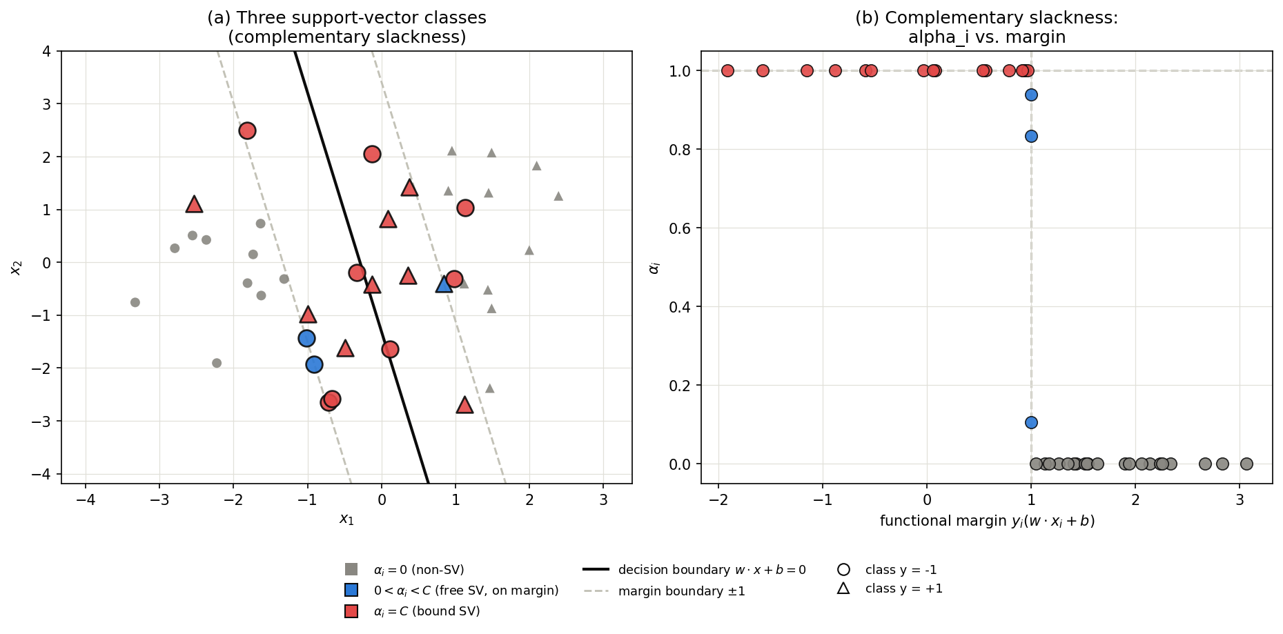
Panel (a) on the left shows the decision boundary, the margin boundaries, and the three types of support vectors (gray = non-SV, blue = free SV, red = bound SV). The free SVs (blue) visibly line up exactly on the dashed margin boundary. Panel (b) on the right plots all 40 points with the functional margin \(y_i(\mathbf{w}\cdot\mathbf{x}_i+b)\) on the x-axis and \(\alpha_i\) on the y-axis: non-SVs sit on the horizontal line \(\alpha_i=0\) (margin \(>1\) ), free SVs sit on the vertical line at margin \(=1\) , and bound SVs sit on the horizontal line \(\alpha_i=C=1\) — exactly the three regions defined by complementary slackness (9).
Kernel Trick
Since the dual (10)-(11) has data appearing only through inner products \(\mathbf{x}_i \cdot \mathbf{x}_j\) , replacing the inner product with a kernel function \(K(\mathbf{x}_i, \mathbf{x}_j) = \phi(\mathbf{x}_i) \cdot \phi(\mathbf{x}_j)\) enables nonlinear classification without explicitly computing the mapping \(\phi\) .
| Kernel | Definition | Use Case |
|---|---|---|
| Linear | \(K(\mathbf{x}, \mathbf{y}) = \mathbf{x} \cdot \mathbf{y}\) | Linearly separable data |
| RBF (Gaussian) | \(K(\mathbf{x}, \mathbf{y}) = \exp(-\gamma\|\mathbf{x}-\mathbf{y}\|^2)\) | Most versatile |
| Polynomial | \(K(\mathbf{x}, \mathbf{y}) = (\gamma \mathbf{x} \cdot \mathbf{y} + r)^d\) | Feature interactions |
Not every two-argument function can serve as a kernel: the necessary and sufficient condition (Mercer’s theorem) is that the Gram matrix over any finite set of data points be positive semi-definite. The numerical verification of this condition, an empirical demonstration that the RBF kernel corresponds to an infinite-dimensional feature map via Random Fourier Features, and a quantitative study of the underfitting/overfitting transition in \(\gamma\) , are all covered in depth in the follow-up article SVM Kernel Design: Mercer’s Theorem, Gram Matrix Positive-Definiteness, and Random Fourier Features .
Python Implementation
import numpy as np
import matplotlib.pyplot as plt
from sklearn.svm import SVC
from sklearn.datasets import make_moons
from sklearn.model_selection import train_test_split
from sklearn.preprocessing import StandardScaler
from sklearn.metrics import accuracy_score

X, y = make_moons(n_samples=300, noise=0.2, random_state=42)
X_train, X_test, y_train, y_test = train_test_split(X, y, test_size=0.3,
                                                      random_state=42)
scaler = StandardScaler()
X_train = scaler.fit_transform(X_train)
X_test = scaler.transform(X_test)

kernels = ['linear', 'rbf', 'poly']
fig, axes = plt.subplots(1, 3, figsize=(15, 4))

for ax, kernel in zip(axes, kernels):
    clf = SVC(kernel=kernel, C=1.0, gamma='scale')
    clf.fit(X_train, y_train)
    acc = accuracy_score(y_test, clf.predict(X_test))

    xx, yy = np.meshgrid(np.linspace(-3, 3, 200), np.linspace(-3, 3, 200))
    Z = clf.decision_function(np.c_[xx.ravel(), yy.ravel()]).reshape(xx.shape)

    ax.contourf(xx, yy, Z, levels=[-1, 0, 1], alpha=0.2, colors=['blue', 'red'])
    ax.contour(xx, yy, Z, levels=[-1, 0, 1], colors='k', linestyles=['--', '-', '--'])
    ax.scatter(X_train[:, 0], X_train[:, 1], c=y_train, cmap='bwr', s=20, alpha=0.6)

    sv = clf.support_vectors_
    ax.scatter(sv[:, 0], sv[:, 1], s=80, facecolors='none', edgecolors='k', linewidths=1.5)

    ax.set_title(f'{kernel} (acc={acc:.3f})')
    ax.set_xlim(-3, 3)
    ax.set_ylim(-3, 3)

plt.tight_layout()
plt.show()
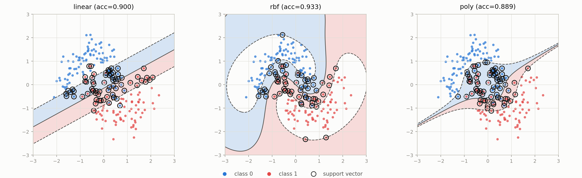
On the held-out test set for the make_moons crescent-shaped data, the linear kernel reached 0.900 accuracy, the RBF kernel 0.933, and the polynomial kernel 0.889. The linear kernel can only draw a straight boundary, so it misclassifies points along the curved parts of the crescents, while the RBF kernel learns a smooth boundary that follows the nonlinear structure of the data and achieves the best accuracy of the three here.
Hyperparameters
C (Regularization)
- Large C: Small margin, strict misclassification penalty → overfitting risk
- Small C: Large margin, tolerates some errors → underfitting risk
As equation (8), \(\mu_i = C - \alpha_i\) , shows, \(C\) is itself the upper bound on \(\alpha_i\) , and directly controls the fraction of points that can become bound support vectors (\(\alpha_i=C\) ).
gamma (RBF Kernel)
- Large gamma: Narrow influence per sample → complex boundary, overfitting
- Small gamma: Wide influence → smooth boundary
from sklearn.model_selection import GridSearchCV

param_grid = {'C': [0.1, 1, 10, 100], 'gamma': [1, 0.1, 0.01, 0.001]}
grid = GridSearchCV(SVC(kernel='rbf'), param_grid, cv=5, scoring='accuracy')
grid.fit(X_train, y_train)
print(f"Best params: {grid.best_params_}, Score: {grid.best_score_:.3f}")
Further Topic: Robustifying the Soft-Margin Loss
The soft-margin penalty \(C\sum_i \xi_i\) is, in essence, the sum of the hinge loss \(\max(0, 1 - y_i f(\mathbf{x}_i))\) . Because the hinge loss grows without bound as points move further from the margin, it can be sensitive to label noise and outliers. Zhang & Yang (2023) proposed a Bounded Quantile Loss that caps this growth, and showed theoretically that classifiers and regressors built on it (BQ-SVM and BQ-SVR) retain Fisher consistency and a generalization error bound. Because the resulting loss is non-convex, they optimize it via the concave-convex procedure (CCCP), decomposing the problem into a difference of convex functions. The soft-margin formulation with \(C\) and \(\xi_i\) is exactly the starting point for this kind of loss-function extension.
SVM Strengths and Limitations
| Strengths | Limitations |
|---|---|
| Strong in high dimensions | Slow on large data (\(O(n^2)\) -\(O(n^3)\) ) |
| Nonlinear via kernels | Probability output requires extra processing |
| Resistant to overfitting | Feature scaling is mandatory |
| Decision boundary from SVs only | Multiclass is indirect (OvO or OvR) |
Related Articles
- SVM Kernel Design in Python: Mercer’s Theorem, Gram Matrix Positive-Definiteness, and Random Fourier Features - A follow-up examining why the kernel trick used here is mathematically valid, grounded in Mercer’s theorem, with the RBF kernel’s infinite dimensionality demonstrated numerically via Random Fourier Features.
- Ensemble Learning: From Decision Trees to Random Forest and Gradient Boosting - Alternative classification methods including Random Forest and GBDT.
- Understanding Self-Attention from Scratch: Math and Python Implementation - Similarity between kernel tricks and Attention.
- k-means and GMM: Clustering Theory and Python Implementation - Contrast supervised classification with unsupervised structure discovery.
- Bayesian Optimization: Fundamentals and Python Implementation - Automate SVM hyperparameter tuning (C, gamma).
- Bayesian Linear Regression: From Least Squares to Bayesian Estimation - Useful comparison between Bayesian regression and SVR.
- Cross-Entropy Method: A Practical Monte Carlo Optimization Technique - Alternative optimization approach for comparison.
- Gaussian Process Regression: Theory and Python Implementation - Uses the same RBF kernel as SVM, but offers probabilistic predictions and uncertainty estimates as a complementary approach.
- Machine Learning Hub for Time-Series Forecasting, Classification, and Anomaly Detection - Hub for choosing among classifiers, including SVM, based on task and data characteristics.
- Time-Series Anomaly Detection: From Statistical Methods to Kalman Filter - Extends decision-boundary classification toward unsupervised anomaly detection such as One-Class SVM.
References
- Vapnik, V. N. (1995). The Nature of Statistical Learning Theory. Springer.
- Cortes, C., & Vapnik, V. (1995). “Support-vector networks”. Machine Learning, 20(3), 273-297.
- Boyd, S., & Vandenberghe, L. (2004). Convex Optimization. Cambridge University Press. Chapter 5 (Duality).
- Zhang, J., & Yang, H. (2023). “Bounded quantile loss for robust support vector machines-based classification and regression”. Expert Systems with Applications, 242, 122759.
- scikit-learn SVM documentation