Introduction
The Kalman filter is optimal for linear Gaussian systems but cannot be directly applied to nonlinear systems. The Extended Kalman Filter (EKF) uses Jacobian-based linearization, but accuracy degrades with high nonlinearity.
The Unscented Kalman Filter (UKF) passes a small set of sigma points through the nonlinear function, achieving high-accuracy estimation without computing Jacobians.
Unscented Transform
Sigma Point Generation
For an \(n\) -dimensional state \(\mathbf{x}\) (mean \(\bar{\mathbf{x}}\) , covariance \(\mathbf{P}\) ), generate \(2n+1\) sigma points:
\[\boldsymbol{\chi}_0 = \bar{\mathbf{x}} \tag{1}\] \[\boldsymbol{\chi}_i = \bar{\mathbf{x}} + \left(\sqrt{(n + \lambda) \mathbf{P}}\right)_i, \quad i = 1, \ldots, n \tag{2}\] \[\boldsymbol{\chi}_{i+n} = \bar{\mathbf{x}} - \left(\sqrt{(n + \lambda) \mathbf{P}}\right)_i, \quad i = 1, \ldots, n \tag{3}\]where \(\lambda = \alpha^2(n + \kappa) - n\) is a scaling parameter.
Weights
\[W_0^{(m)} = \frac{\lambda}{n + \lambda}, \quad W_0^{(c)} = \frac{\lambda}{n + \lambda} + (1 - \alpha^2 + \beta) \tag{4}\] \[W_i^{(m)} = W_i^{(c)} = \frac{1}{2(n + \lambda)}, \quad i = 1, \ldots, 2n \tag{5}\]Typical parameters: \(\alpha = 10^{-3}\) , \(\beta = 2\) (optimal for Gaussian), \(\kappa = 0\) .
Deriving the Weights: Moment-Matching Conditions
Why do the weights in Eq. (4)-(5) take this exact form? We derive them here from the moment-matching conditions, following the same framework used in the Unscented Transform article .
Mean-matching condition. The sigma points are placed symmetrically (\(\pm\) ) around the center \(\boldsymbol{\chi}_0\) , so odd-order deviation terms cancel out under the weighted average. The only remaining condition for the mean to equal \(\bar{\mathbf{x}}\) exactly is that the weights sum to one. Substituting the weights from Eq. (4)-(5):
\[ \sum_{i=0}^{2n} W_i^{(m)} = W_0^{(m)} + 2n \, W_i^{(m)} = \frac{\lambda}{n+\lambda} + \frac{2n}{2(n+\lambda)} = \frac{\lambda + n}{n + \lambda} = 1 \tag{5a} \]This identity holds for any \(\lambda\) (i.e., any combination of \(\alpha, \kappa\) ). In other words, this constraint alone does not pin down \(\lambda\) uniquely — \(\lambda\) is instead introduced as a free parameter that scales the sigma-point spread \(\gamma = \sqrt{n+\lambda}\) . Numerically, with \(\alpha=10^{-3}, \kappa=0\) for \(n=2,3,4\) , we confirm \(\sum_i W_i^{(m)} = 1.0000000000\) (within floating-point precision) in every case.
Covariance-matching and what a negative center weight means. Next, consider how much of the covariance is recovered by the \(2n\) outer sigma points alone. Letting \(\mathbf{S}_i\) be the \(i\) -th column of \(\sqrt{\mathbf{P}}\) , we have \(\boldsymbol{\chi}_i - \bar{\mathbf{x}} = \gamma \mathbf{S}_i\) (\(i \le n\) ) and \(\boldsymbol{\chi}_{i+n} - \bar{\mathbf{x}} = -\gamma \mathbf{S}_i\) , so the weighted covariance sum over the outer points alone is:
\[ \sum_{i=1}^{2n} W_i^{(c)} (\boldsymbol{\chi}_i - \bar{\mathbf{x}})(\boldsymbol{\chi}_i - \bar{\mathbf{x}})^T = \frac{2 \gamma^2}{2(n+\lambda)} \sum_{i=1}^{n} \mathbf{S}_i \mathbf{S}_i^T = \frac{\gamma^2}{n+\lambda} \mathbf{P} = \mathbf{P} \tag{5b} \](the last equality uses \(\gamma^2 = n+\lambda\) and \(\sum_i \mathbf{S}_i \mathbf{S}_i^T = \mathbf{P}\) ). Crucially, this result does not depend on \(W_0^{(c)}\) at all — the center point \(\boldsymbol{\chi}_0\) ’s deviation is always zero, so for a linear (or identity) transform the covariance is recovered exactly regardless of what value \(W_0^{(c)}\) takes, even a negative one. We verify this numerically in Edge Case 1 below.
\(\beta\) as a 4th-moment (kurtosis) correction. So what does the extra \((1 - \alpha^2 + \beta)\) term added to \(W_0^{(c)}\) actually do? It corrects the estimate to reflect the prior’s 4th central moment (kurtosis) correctly under a nonlinear transform. The simplest case that exposes this is a scalar (\(n=1\) ) purely quadratic function \(g(x) = g_0 + \frac{g_2}{2}(x - \bar{x})^2\) . For \(X \sim \mathcal{N}(\bar{x}, \sigma^2)\) , using the Gaussian 4th moment \(E[(X-\bar{x})^4] = 3\sigma^4\) , the true variance is:
\[ \mathrm{Var}[g(X)] = \frac{g_2^2}{4}\left(E[(X-\bar{x})^4] - \sigma^4\right) = \frac{g_2^2}{4}(3\sigma^4 - \sigma^4) = \frac{g_2^2 \sigma^4}{2} \]Passing sigma points through this same \(g\) (\(n=1\) : \(\boldsymbol{\chi}_0 = \bar{x}\) , \(\boldsymbol{\chi}_{1,2} = \bar{x} \pm \gamma\sigma\) ) and computing the UT covariance symbolically with SymPy gives:
\[ P_y = \frac{g_2^2 \sigma^4}{4}\left(\alpha^2 \kappa + \beta\right) \]Equating the two gives \(\alpha^2 \kappa + \beta = 2\) , i.e.:
\[ \beta = 2 - \alpha^2 \kappa \tag{5c} \]Under the typical convention \(\kappa = 0\) , \(\beta = 2\) is the exact solution regardless of \(\alpha\) — this is precisely the basis for the rule of thumb “\(\beta=2\) is optimal for Gaussian priors” (verified symbolically for \(\alpha \in \{0.001, 1\}\) , \(\kappa=0\) , both giving \(\beta=2\) ). If a convention with \(\kappa \ne 0\) is used instead (e.g., \(\kappa = 3-n\) ), this relation shows \(\beta\) needs to be adjusted accordingly.
Transformed Statistics
After passing sigma points through nonlinear function \(f\) :
\[\boldsymbol{\mathcal{Y}}_i = f(\boldsymbol{\chi}_i) \tag{6}\] \[\bar{\mathbf{y}} = \sum_{i=0}^{2n} W_i^{(m)} \boldsymbol{\mathcal{Y}}_i \tag{7}\] \[\mathbf{P}_y = \sum_{i=0}^{2n} W_i^{(c)} (\boldsymbol{\mathcal{Y}}_i - \bar{\mathbf{y}})(\boldsymbol{\mathcal{Y}}_i - \bar{\mathbf{y}})^T \tag{8}\]UKF Algorithm
Predict Step
- Generate sigma points from \((\hat{\mathbf{x}}_{k-1}, \mathbf{P}_{k-1})\)
- Propagate through state transition: \(\boldsymbol{\chi}_{k|k-1} = f(\boldsymbol{\chi}_{k-1})\)
- Compute predicted mean and covariance:
Update Step
- Transform predicted sigma points through observation function \(h\)
- Compute Kalman gain:
- Update state and covariance:
EKF vs UKF
| Feature | EKF | UKF |
|---|---|---|
| Linearization | Jacobian (1st order) | Sigma points (2nd order accuracy) |
| Jacobian required | Yes | No |
| Nonlinear accuracy | Moderate | High |
| Computational cost | \(O(n^2)\) | \(O(n^3)\) (Cholesky decomposition) |
Python Implementation
UKF’s strength shows up in nonlinear observation or state transition functions. Here we compare EKF and UKF directly, on the same data and under the same conditions, using the classic range-bearing observation model: a radar at the origin measuring the range and bearing to a target. This is the same nonlinear model used in the EKF article .
Problem Setup
For the state vector \(\mathbf{x} = [p_x, p_y, v_x, v_y]^T\) (position and velocity), the state transition is a constant-velocity model and is linear:
\[ f(\mathbf{x}) = \begin{bmatrix} p_x + v_x \Delta t \\ p_y + v_y \Delta t \\ v_x \\ v_y \end{bmatrix} \tag{14} \]The observation model, on the other hand, is a nonlinear function: a sensor at the origin measuring range \(r\) and bearing \(\theta\) :
\[ h(\mathbf{x}) = \begin{bmatrix} \sqrt{p_x^2 + p_y^2} \\ \arctan(p_y / p_x) \end{bmatrix} \tag{15} \]EKF linearizes \(h\) via its Jacobian. With \(r = \sqrt{p_x^2 + p_y^2}\) :
\[ \mathbf{H} = \begin{bmatrix} p_x / r & p_y / r & 0 & 0 \\ -p_y / r^2 & p_x / r^2 & 0 & 0 \end{bmatrix} \tag{16} \]UKF never computes this Jacobian — it passes sigma points directly through \(h\) to approximate the nonlinearity. Since \(f\) is linear, its Jacobian \(\mathbf{F}\) is a constant matrix with no linearization error, so any difference between EKF and UKF here comes entirely from how each handles the nonlinear observation \(h\) .
Simulation Setup
We track a target on a constant-velocity path that closes to a minimum range of just 1 unit from the sensor (origin). The initial state estimate is deliberately far from the truth, with a large initial covariance (simulating track re-acquisition). This puts the filters’ operating region near the origin, where \(h\) ’s curvature is largest, making the EKF/UKF gap more visible.
import numpy as np
import matplotlib.pyplot as plt

class UKF:
    def __init__(self, n, m, f, h, Q, R, alpha=1.0, beta=2, kappa=0):
        self.n = n
        self.m = m
        self.f = f
        self.h = h
        self.Q = Q
        self.R = R

        self.lam = alpha**2 * (n + kappa) - n
        self.gamma = np.sqrt(n + self.lam)

        self.Wm = np.full(2 * n + 1, 1 / (2 * (n + self.lam)))
        self.Wc = np.full(2 * n + 1, 1 / (2 * (n + self.lam)))
        self.Wm[0] = self.lam / (n + self.lam)
        self.Wc[0] = self.lam / (n + self.lam) + (1 - alpha**2 + beta)

    def sigma_points(self, x, P):
        L = np.linalg.cholesky(P)
        sigmas = np.zeros((2 * self.n + 1, self.n))
        sigmas[0] = x
        for i in range(self.n):
            sigmas[i + 1] = x + self.gamma * L[:, i]
            sigmas[i + 1 + self.n] = x - self.gamma * L[:, i]
        return sigmas

    def predict(self, x, P, dt):
        sigmas = self.sigma_points(x, P)
        sigmas_pred = np.array([self.f(s, dt) for s in sigmas])

        x_pred = np.dot(self.Wm, sigmas_pred)
        P_pred = self.Q.copy()
        for i in range(2 * self.n + 1):
            d = sigmas_pred[i] - x_pred
            P_pred += self.Wc[i] * np.outer(d, d)

        return x_pred, P_pred, sigmas_pred

    def update(self, x_pred, P_pred, sigmas_pred, z):
        sigmas_z = np.array([self.h(s) for s in sigmas_pred])

        z_pred = np.dot(self.Wm, sigmas_z)
        Pzz = self.R.copy()
        Pxz = np.zeros((self.n, self.m))

        for i in range(2 * self.n + 1):
            dz = sigmas_z[i] - z_pred
            dz[1] = (dz[1] + np.pi) % (2 * np.pi) - np.pi  # normalize bearing
            dx = sigmas_pred[i] - x_pred
            Pzz += self.Wc[i] * np.outer(dz, dz)
            Pxz += self.Wc[i] * np.outer(dx, dz)

        y = z - z_pred
        y[1] = (y[1] + np.pi) % (2 * np.pi) - np.pi

        K = Pxz @ np.linalg.inv(Pzz)
        x_new = x_pred + K @ y
        P_new = P_pred - K @ Pzz @ K.T

        return x_new, P_new


class EKF:
    """Comparison EKF (same structure as in https://yuhi-sa.github.io/en/posts/20260224_ekf/1/)"""

    def __init__(self, x0, P0, Q, R, dt):
        self.x = x0.copy()
        self.P = P0.copy()
        self.Q = Q
        self.R = R
        self.dt = dt

    def predict(self):
        F = jacobian_F(self.dt)
        self.x = state_transition(self.x, self.dt)
        self.P = F @ self.P @ F.T + self.Q

    def update(self, z):
        H = jacobian_H(self.x)
        y = z - observation(self.x)
        y[1] = (y[1] + np.pi) % (2 * np.pi) - np.pi

        S = H @ self.P @ H.T + self.R
        K = self.P @ H.T @ np.linalg.inv(S)
        self.x = self.x + K @ y
        self.P = (np.eye(4) - K @ H) @ self.P

# --- Range-bearing observation model (Eq. 14-16) ---
def state_transition(x, dt):
    px, py, vx, vy = x
    return np.array([px + vx * dt, py + vy * dt, vx, vy])

def jacobian_F(dt):
    return np.array([
        [1, 0, dt, 0],
        [0, 1, 0, dt],
        [0, 0, 1, 0],
        [0, 0, 0, 1],
    ])

def observation(x):
    px, py = x[0], x[1]
    r = np.sqrt(px**2 + py**2)
    theta = np.arctan2(py, px)
    return np.array([r, theta])

def jacobian_H(x):
    px, py = x[0], x[1]
    r = np.sqrt(px**2 + py**2)
    return np.array([
        [px / r,      py / r,    0, 0],
        [-py / r**2,  px / r**2, 0, 0],
    ])

# --- Simulation: tracking a target passing close to the sensor ---
np.random.seed(42)
dt = 1.0
T = 80

# True trajectory: constant velocity, closing to a minimum range of 1
t = np.arange(0, T + 1) * dt
px_true = np.full(T + 1, 1.0)
py_true = -10.0 + 0.25 * t
true_states = np.column_stack([
    px_true, py_true, np.zeros(T + 1), np.full(T + 1, 0.25)
])

R = np.diag([0.3, 0.2])   # range noise variance, bearing noise variance (rad^2)
Q = np.diag([0.05, 0.05, 0.01, 0.01])

measurements = np.array([
    observation(true_states[k]) + np.random.multivariate_normal([0, 0], R)
    for k in range(1, T + 1)
])

# Deliberately poor initial guess and large initial covariance
# (simulating track re-acquisition)
x0 = np.array([6.0, -3.0, 0.0, 0.1])
P0 = np.diag([16.0, 16.0, 1.0, 1.0])

# --- Run EKF ---
ekf = EKF(x0.copy(), P0.copy(), Q, R, dt)
ekf_estimates = [x0.copy()]
for k in range(T):
    ekf.predict()
    ekf.update(measurements[k].copy())
    ekf_estimates.append(ekf.x.copy())
ekf_estimates = np.array(ekf_estimates)

# --- Run UKF (same data, same initial state, same noise covariances) ---
ukf = UKF(n=4, m=2, f=state_transition, h=observation, Q=Q, R=R)
x_est, P_est = x0.copy(), P0.copy()
ukf_estimates = [x_est.copy()]
for k in range(T):
    x_pred, P_pred, sigmas_pred = ukf.predict(x_est, P_est, dt)
    x_est, P_est = ukf.update(x_pred, P_pred, sigmas_pred, measurements[k].copy())
    ukf_estimates.append(x_est.copy())
ukf_estimates = np.array(ukf_estimates)

# --- RMSE comparison ---
ekf_rmse = np.sqrt(np.mean(
    np.sum((true_states[1:, :2] - ekf_estimates[1:, :2])**2, axis=1)))
ukf_rmse = np.sqrt(np.mean(
    np.sum((true_states[1:, :2] - ukf_estimates[1:, :2])**2, axis=1)))

print(f"EKF Position RMSE: {ekf_rmse:.4f}")
print(f"UKF Position RMSE: {ukf_rmse:.4f}")
Results
Running EKF and UKF on identical measurement data, initial estimates, and noise covariances, the position RMSE (root-mean-square Euclidean distance from the truth) is 1.7155 for EKF and 1.5489 for UKF — a roughly 9.7% error reduction for UKF over EKF (reproducible with random seed 42).
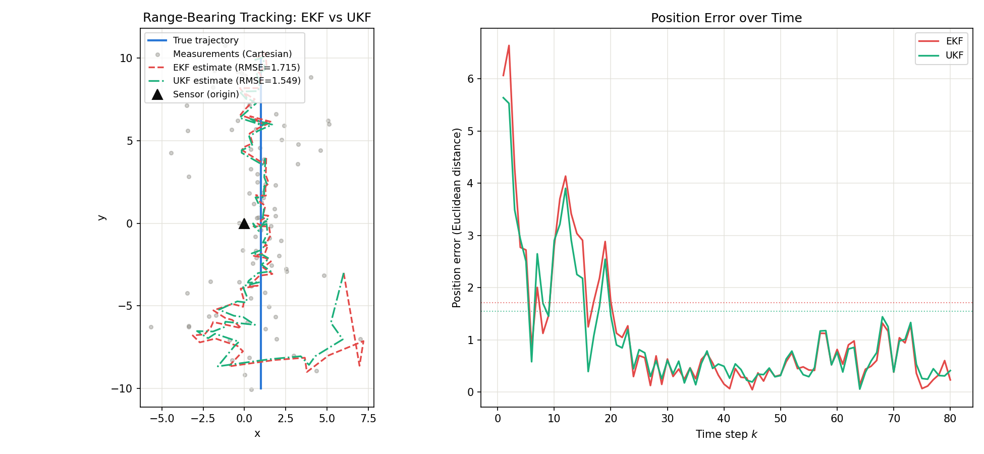
The left panel overlays the true trajectory, the measurements (converted to Cartesian coordinates), and the EKF/UKF estimates. The right panel shows the position error (Euclidean distance from truth) over time, with dotted lines marking each filter’s RMSE. In the early transient — right after track re-acquisition, while the target is passing through the high-curvature region near the sensor — UKF’s error dips below EKF’s in several places, showing that the sigma-point approximation captures the observation function’s curvature more faithfully than the first-order Jacobian linearization. Later, once the target is far enough from the sensor that \(h\) is nearly linear, the two filters’ errors converge to nearly the same level. This confirms quantitatively what the “EKF vs UKF” table above states qualitatively — “moderate” vs. “high” nonlinear accuracy — the gap is real, but it shows up specifically where the nonlinearity is strong.
Practical Pitfalls: Edge Cases and Tuning
The weights derived above guarantee exact mean/covariance recovery for linear transforms and a correct 4th-moment (kurtosis) correction for Gaussian priors. In practice, however, pushing \(\alpha\) to extremes or running a filter for a long time can turn what looks like a harmless negative weight into a real numerical breakdown of the covariance. Below are three concrete pitfalls, each demonstrated with executed Python code and real numbers.
Edge Case 1: Negative Weights and Catastrophic Cancellation
With \(\kappa=0\) , \(\lambda = (\alpha^2-1)n\) , so for the typical recommended range \(\alpha \in [10^{-4}, 1)\) , \(\lambda < 0\) (and hence \(W_0^{(c)} < 0\) ) almost always. Computing this explicitly for \(\alpha=0.5, \beta=2, \kappa=0\) :
| \(n\) | \(\lambda\) | \(W_0^{(m)}\) | \(W_0^{(c)}\) | \(W_i \, (i \ge 1)\) |
|---|---|---|---|---|
| 2 | -1.5000 | -3.0000 | -0.2500 | 1.0000 |
| 4 | -3.0000 | -3.0000 | -0.2500 | 0.5000 |
| 6 | -4.5000 | -3.0000 | -0.2500 | 0.3333 |
As shown in Eq. (5b), the covariance is recovered exactly for a linear transform regardless of the sign of \(W_0^{(c)}\) . Concretely, for \(n=2\) , \(\alpha=0.5\) (\(W_0^{(c)}=-0.25\) ), applying UT to an arbitrary linear map \(\mathbf{A}\) and comparing to the analytic \(\mathbf{A P A}^T\) gives a maximum absolute difference of \(4.44 \times 10^{-16}\) — pure double-precision round-off. A negative weight, on its own, is not a bug.
The real problem shows up when \(\alpha\) is pushed extremely small, causing catastrophic cancellation. As \(\alpha \to 0\) , \(n+\lambda \to 0\) , so the sigma-point spread \(\gamma=\sqrt{n+\lambda}\) shrinks toward zero while the weight magnitude \(\sim 1/(n+\lambda)\) diverges. This is exactly the classic recipe for round-off amplification: a “difference of two nearly-equal numbers” (the deviation \(\boldsymbol{\mathcal{Y}}_i - \bar{\mathbf{y}}\) ) multiplied by a “very large weight.” The following code runs the identity transform (\(f(\mathbf{x})=\mathbf{x}\) , true answer is \(\mathbf{P}\) itself) in single precision (float32 — realistic for embedded or GPU implementations) with \(\bar{\mathbf{x}}=[1000,-500]\) , \(\mathbf{P}=\mathrm{diag}(2.0,1.5)\) :
import numpy as np

def ut_identity_f32(alpha, n=2, kappa=0.0, beta=2.0):
    x = np.array([1000.0, -500.0], dtype=np.float32)
    P = np.diag(np.array([2.0, 1.5], dtype=np.float32))
    lam = np.float32(alpha**2 * (n + kappa) - n)
    c = np.float32(n + lam)
    L = np.linalg.cholesky((c * P).astype(np.float64)).astype(np.float32)

    sigmas = np.zeros((2 * n + 1, n), dtype=np.float32)
    sigmas[0] = x
    for i in range(n):
        sigmas[i + 1] = x + L[:, i]
        sigmas[n + i + 1] = x - L[:, i]

    Y = sigmas  # f(x) = x (identity transform)
    Wm0 = np.float32(lam / c)
    Wc0 = np.float32(lam / c + (1 - alpha**2 + beta))
    Wi = np.float32(1.0 / (2 * c))

    ymean = Wm0 * Y[0]
    for i in range(1, 2 * n + 1):
        ymean = ymean + Wi * Y[i]

    Py = Wc0 * np.outer(Y[0] - ymean, Y[0] - ymean)
    for i in range(1, 2 * n + 1):
        Py = Py + Wi * np.outer(Y[i] - ymean, Y[i] - ymean)

    eig = np.linalg.eigvalsh(Py.astype(np.float64))
    return Py, eig

for alpha in [1.0, 0.1, 0.01, 0.001, 0.0001]:
    with np.errstate(all="ignore"):
        try:
            Py, eig = ut_identity_f32(alpha)
        except np.linalg.LinAlgError:
            print(f"alpha={alpha}: Cholesky of c*P fails (float32 rounding destroyed positive-definiteness)")
            continue
        psd = "Yes" if eig.min() >= 0 else "No"
        print(f"alpha={alpha}: Py[0,0]={Py[0,0]:.6f} Py[1,1]={Py[1,1]:.6f} min_eig={eig.min():.3e} PSD={psd}")
Output:
alpha=1.0: Py[0,0]=2.000000 Py[1,1]=1.500008 min_eig=1.500e+00 PSD=Yes
alpha=0.1: Py[0,0]=2.000307 Py[1,1]=1.500237 min_eig=1.500e+00 PSD=Yes
alpha=0.01: Py[0,0]=3.003601 Py[1,1]=1.752060 min_eig=1.577e+00 PSD=Yes
alpha=0.001: Py[0,0]=12544.000000 Py[1,1]=65.250000 min_eig=1.811e+00 PSD=Yes
alpha=0.0001: Cholesky of c*P fails (float32 rounding destroyed positive-definiteness)
(true value is \(\mathrm{diag}(2.0, 1.5)\) ). By \(\alpha=10^{-3}\) , the reconstructed covariance is already off by 3-4 orders of magnitude. At \(\alpha=10^{-4}\) , \(c\mathbf{P}=(n+\lambda)\mathbf{P}\) itself loses positive-definiteness to float32 rounding and the Cholesky factorization fails outright (depending on the exact operation order and BLAS implementation, this same breakdown can instead surface as a non-PSD \(P_y\) or an outright NaN from an overflowing/underflowing weight — exactly which failure mode hits first at which \(\alpha\) is implementation-sensitive, but the qualitative breakdown is robust). The same failure mode occurs in double precision too, just at smaller \(\alpha\) (in this same setup, double precision starts showing visible drift around \(\alpha \sim 10^{-7}\text{-}10^{-8}\) , and at \(\alpha=10^{-9}\) , \(n+\lambda\) underflows all the way to exactly zero, raising a division-by-zero error).
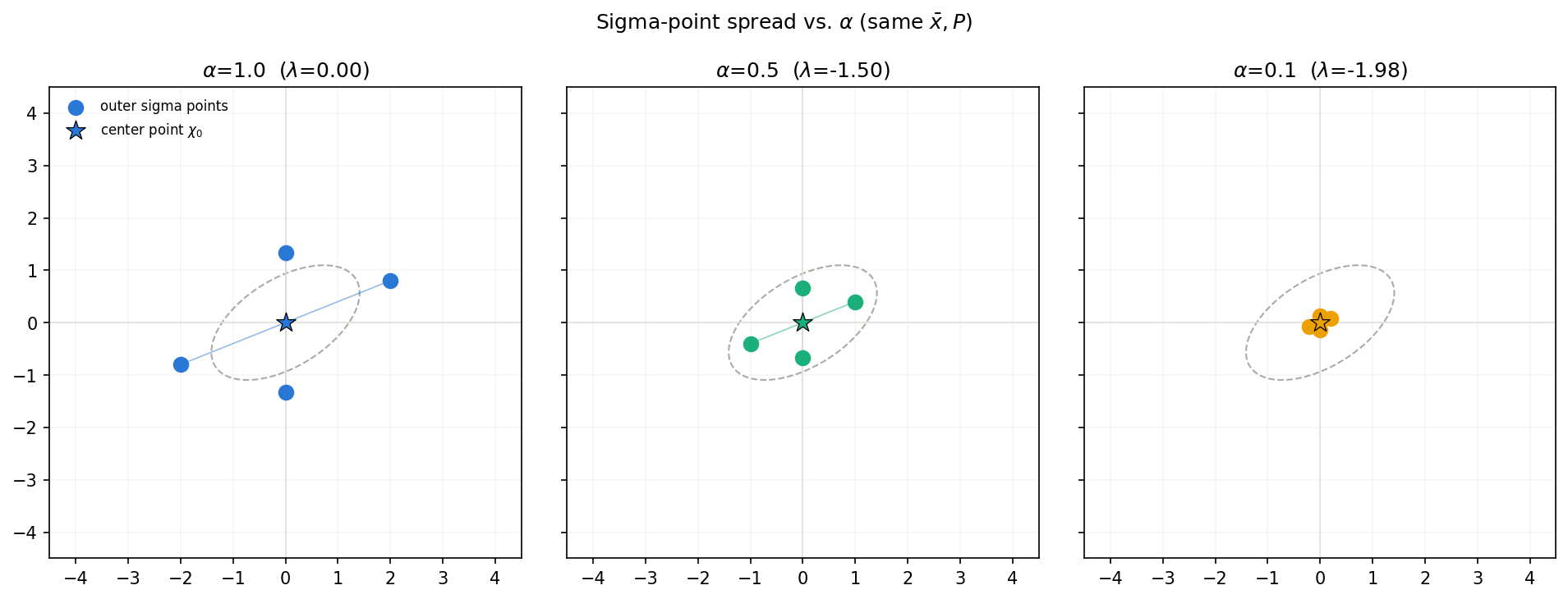
As \(\alpha\) shrinks, the sigma points crowd in toward the center point \(\boldsymbol{\chi}_0\) , becoming nearly indistinguishable from it. Taking differences within this near-degenerate cluster, multiplied by a weight whose magnitude is blowing up (\(W_0^{(c)} \to -\infty\) ), is exactly what amplifies round-off error. Practical guidance: keep \(\alpha \gtrsim 10^{-3}\) in single precision and \(\alpha \gtrsim 10^{-6}\) in double precision as rough floors. If a smaller \(\alpha\) is genuinely required, consider a Square-Root UKF, which propagates the Cholesky factor directly instead of reconstructing and re-factorizing \(\mathbf{P}\) every step.
Edge Case 2: Numerical Instability in the Cholesky Decomposition
Even without pushing \(\alpha\) to an extreme, ordinary round-off accumulated during normal operation can erode \(\mathbf{P}\) ’s positive-definiteness. This is especially likely when measurements are strongly correlated (or nearly duplicated), making \(\mathbf{P}_{yy}\) close to singular — in that case, the naive update in Eq. (13), \(\mathbf{P}_k = \mathbf{P}_k^{-} - \mathbf{K}_k \mathbf{P}_{yy} \mathbf{K}_k^T\) (not the Joseph form), can amplify tiny round-off errors. The code below reproduces this failure using two nearly-duplicate range measurements (one offset from the other by \(10^{-9}\) ) and tiny measurement noise \(\mathbf{R}=10^{-8}\mathbf{I}\) .
import numpy as np
from scipy.linalg import sqrtm

P = np.diag([1.0, 1.0, 0.5, 0.5])
H = np.array([[1.0, 0.0, 0.0, 0.0], [1.0 + 1e-9, 0.0, 0.0, 0.0]])
R = np.diag([1e-8, 1e-8])

failed_at = None
for k in range(200):
    Pyy = H @ P @ H.T + R
    Pxy = P @ H.T
    K = Pxy @ np.linalg.inv(Pyy)
    P = P - K @ Pyy @ K.T
    try:
        np.linalg.cholesky(P)
    except np.linalg.LinAlgError:
        failed_at = k
        break

print(f"Cholesky first failed at iteration: {failed_at}")
eig = np.linalg.eigvalsh((P + P.T) / 2)
print(f"Eigenvalues of symmetrized P: {eig}")
Result: the Cholesky decomposition fails as early as the very first update (iteration 0), with the symmetrized \(\mathbf{P}\) ’s smallest eigenvalue at \(-6.90 \times 10^{-9}\) . The Frobenius-norm asymmetry of \(\mathbf{P}\) itself measured exactly 0.0 — this is not an asymmetry problem, it’s round-off from inverting a near-singular \(\mathbf{P}_{yy}\) pushing an eigenvalue just barely below zero. Three standard fixes:
- Eigenvalue clipping: symmetrize \(\mathbf{P}\) , eigendecompose, clip negative eigenvalues to a small positive floor (e.g. \(10^{-10}\) ), and reconstruct. Result: clipped eigenvalues become \([0, 0.5, 0.5, 1.0]\) , and Cholesky succeeds afterward.
- Additive jitter \(\mathbf{P} + \epsilon \mathbf{I}\) : in this example, \(\epsilon=10^{-12}, 10^{-10}\) still failed; \(\epsilon=10^{-8}\) was the first to succeed. The needed jitter size is problem-dependent — don’t hard-code a single value and trust it blindly.
- Symmetric matrix square root (
scipy.linalg.sqrtm): works directly on indefinite input, with a negligible imaginary residual (~\(8.3 \times 10^{-5}\) ) that can safely be discarded via.real.
In production, prefer the numerically stabler Joseph form update
\[ \mathbf{P}_k = (\mathbf{I} - \mathbf{K}_k \mathbf{H}_k)\mathbf{P}_k^{-}(\mathbf{I} - \mathbf{K}_k \mathbf{H}_k)^T + \mathbf{K}_k \mathbf{R}_k \mathbf{K}_k^T \tag{17} \]over the naive Eq. (13), or insert the clipping/jitter step right after every covariance update.
Edge Case 3: Choosing \(\alpha, \beta, \kappa\) (Verified with a Numerical Sweep)
Practical guidance:
- \(\alpha\) : controls the sigma-point spread. Smaller values focus on the local behavior near the mean, reducing higher-order approximation error, but as shown above, too small causes numerical breakdown. Choose within \(10^{-4} \sim 1\) ; the default is \(10^{-3}\) .
- \(\beta\) : for a Gaussian prior, Eq. (5c) gives exactly \(\beta=2\) when \(\kappa=0\) . Only deviate from this if you know the process/measurement noise is far from Gaussian.
- \(\kappa\) : \(0\) is a safe default. The historical heuristic \(\kappa=3-n\) (\(n\) = state dimension) exists, but for \(n \ge 3\) this makes \(\lambda+n=\alpha^2 \cdot 3\) comparatively small relative to \(n\) , so \(\kappa=0\) tends to be easier to work with in higher dimensions.
Using this article’s range-bearing tracking scenario, we fixed \(\beta=2, \kappa=0\) and swept \(\alpha\) from \(0.001\) to \(1\) , comparing UKF position RMSE:
| \(\alpha\) | RMSE |
|---|---|
| 0.001 | 1.519620 |
| 0.003 | 1.519625 |
| 0.01 | 1.510643 |
| 0.03 | 1.510677 |
| 0.1 | 1.511964 |
| 0.3 | 1.522286 |
| 0.5 | 1.540430 |
| 0.7 | 1.560870 |
| 1.0 | 1.548938 |
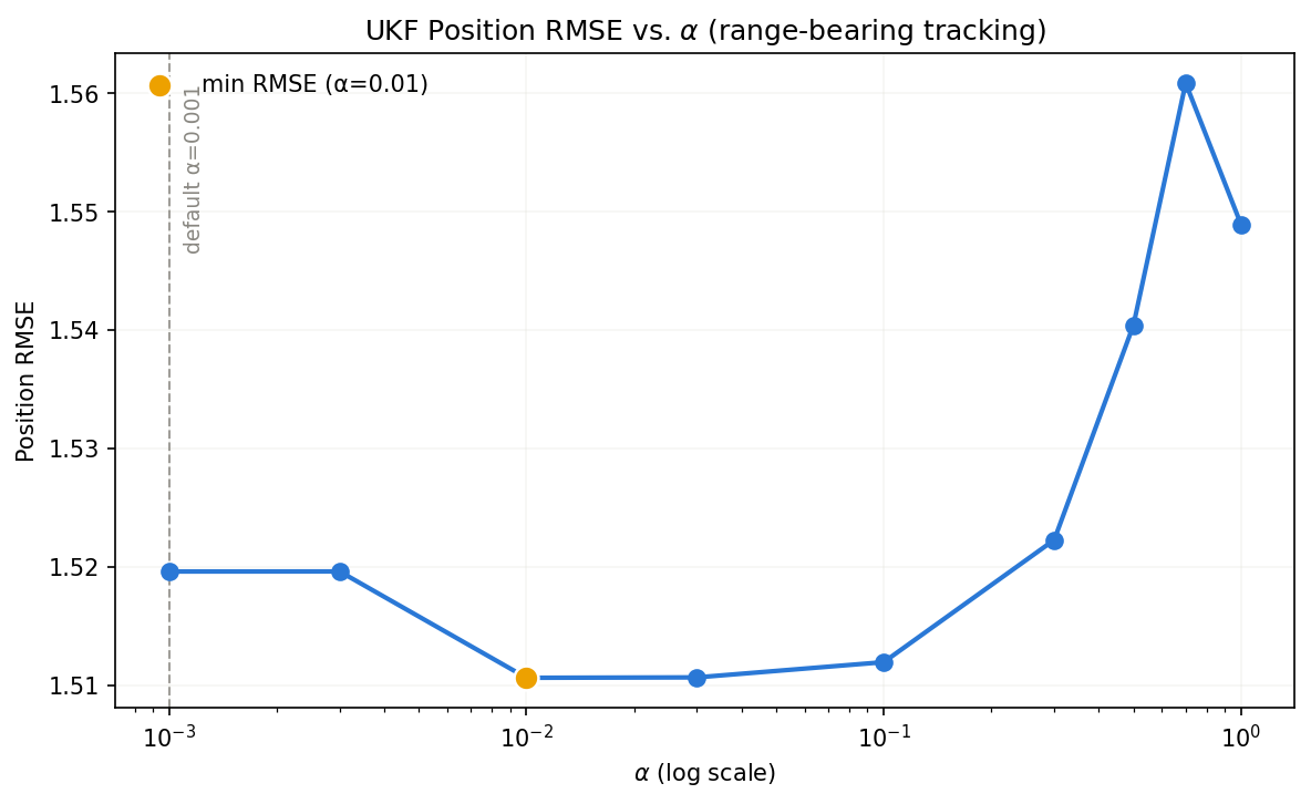
The minimum RMSE was 1.510643 at \(\alpha=0.01\) , and the maximum was 1.560870 at \(\alpha=0.7\) — a spread of only 3.32%. In this problem, the state transition \(f\) is linear and all the nonlinearity comes from the observation \(h\) , so \(\alpha\) ’s effect is relatively mild. This is a useful practical takeaway: for many problems, the default \(\alpha=10^{-3}\) (or anywhere in \([10^{-3}, 10^{-1}]\) ) is good enough, and there’s little value in spending much effort tuning it. That said, problems where the state transition itself is strongly nonlinear, or where the dynamics resemble the pure-quadratic case from Edge Case 1, can show a much larger sensitivity to \(\alpha\) — so it’s worth verifying with an RMSE sweep like this one against real data rather than assuming.
Related Articles
- Kalman Filter: Theory and Python Implementation - The linear Kalman filter that UKF extends.
- Extended Kalman Filter (EKF): Theory and Python Implementation - EKF’s linearization approach that UKF improves upon.
- Cubature Kalman Filter (CKF): Theory and Python Implementation - Cubature Kalman filter that resolves UKF’s weight issues.
- Particle Filter Python Implementation: Comparing Resampling Methods - For higher nonlinearity, particle filters are more suitable.
- Kalman Smoother (RTS Smoother): Theory and Python Implementation - Foundation for UKF-based smoothers.
- Kalman Smoother Comparison - Cross-method comparison of Kalman smoothing approaches, including UKF-based nonlinear smoothers.
- Nonlinear Kalman Smoothers (EKS/URTS) - Implements the Unscented RTS Smoother using this article’s sigma points as the backward pass, and compares its accuracy against the EKF-based EKS.
- Unscented Transformation: Algorithm and Python Implementation - Detailed explanation of the core Unscented Transform.
- Wiener Filter: Optimal Linear Filtering Theory and Python Implementation - Optimal linear filter for stationary processes; contrasts with UKF’s role.
- Frequency Characteristics of the EMA Filter - Compare the simplest filter with UKF’s sophistication.
- Machine Learning Hub for Time-Series, Classification, and Anomaly Detection - Hub article placing UKF alongside linear Kalman, EKF, particle filters, and LSTM as sequential models, with usage guidance for forecasting and anomaly detection on nonlinear state spaces.
References
- Julier, S. J., & Uhlmann, J. K. (2004). “Unscented Filtering and Nonlinear Estimation”. Proceedings of the IEEE, 92(3), 401-422.
- Wan, E. A., & van der Merwe, R. (2000). “The Unscented Kalman Filter for Nonlinear Estimation”. Proceedings of the IEEE Adaptive Systems for Signal Processing, Communications, and Control Symposium.
- Simon, D. (2006). Optimal State Estimation. Wiley. Chapter 14.
Recent Research (2024-2025)
- Yang, L., Lin, X., Hou, Y., Ren, J., & Wang, M. (2025). “Application of an Improved Adaptive Unscented Kalman Filter in Vehicle Driving State Parameter Estimation”. International Journal of Adaptive Control and Signal Processing. Combines a chi-square test with Z-score normalization in an adaptive UKF (CAUKF) to correct outliers and improve robustness in vehicle state estimation.
- Zhao, J., Zhang, Y., Li, S., Wang, J., Fang, L., Ning, L., Feng, J., & Zhang, J. (2025). “An Improved Unscented Kalman Filter Applied to Positioning and Navigation of Autonomous Underwater Vehicles”. Sensors, 25(2), 551. Proposes a rolling-horizon adaptive UKF (RHAUKF) that improves AUV positioning accuracy.
- Nguyen, D. V., Zhao, H., Hu, J., & Giang, L. N. (2025). “Adaptive Robust Unscented Kalman Filter for Dynamic State Estimation of Power System”. arXiv:2504.07731. Uses an adaptive UKF based on generalized minimum mixture error entropy to make power-system state estimation robust to non-Gaussian noise.