Introduction
As discussed in the FFT article , the Fourier transform is a powerful tool for decomposing signals into sinusoidal frequency components. However, it has an inherent limitation: loss of time information.
The Fourier transform tells us “which frequencies are present in the signal as a whole” but not “when those frequencies occurred.” For signals whose frequency content changes over time, such as speech or seismic waves, this limitation is critical.
The Short-Time Fourier Transform (STFT) introduces time localization using a window function, but its fixed window size cannot simultaneously achieve high resolution for both high and low frequencies. The Wavelet Transform solves this problem by providing adaptive resolution in both time and frequency.
This article covers the mathematical foundations of the Continuous Wavelet Transform (CWT) and Discrete Wavelet Transform (DWT), along with Python implementations using PyWavelets.
From Fourier to Wavelet Transform
Limitations of STFT: Fixed Window Size
The STFT segments a signal with a short window and applies the Fourier transform to each segment:
\[\text{STFT}\{x(t)\}(\tau, \omega) = \int_{-\infty}^{\infty} x(t) \, w(t - \tau) \, e^{-j\omega t} \, dt \tag{1}\]where \(w(t)\) is the window function and \(\tau\) is the time shift. The fundamental issue with STFT is that the window size is fixed:
- Short window: Good time resolution, poor frequency resolution
- Long window: Good frequency resolution, poor time resolution
This trade-off is governed by the Heisenberg uncertainty principle. There is a lower bound on the product of time spread \(\Delta t\) and frequency spread \(\Delta f\) :
\[\Delta t \cdot \Delta f \geq \frac{1}{4\pi} \tag{2}\]In STFT, the product \(\Delta t \cdot \Delta f\) is fixed at a constant value. Wavelet transforms maintain this constant product but adaptively redistribute \(\Delta t\) and \(\Delta f\) depending on frequency.
The Wavelet Transform Idea
The key insight of wavelet analysis is to use localized waveforms (wavelets) as basis functions instead of sinusoids. Wavelets have finite temporal extent, naturally providing time localization.
By dilating and compressing the wavelet, different frequency bands can be analyzed at different resolutions:
- Small scale (compressed wavelet): Captures high-frequency components with high time resolution
- Large scale (stretched wavelet): Captures low-frequency components with high frequency resolution
Continuous Wavelet Transform (CWT)
Mother Wavelet
The basis function for the wavelet transform is called the mother wavelet \(\psi(t)\) . It must satisfy two conditions:
- Finite energy: \(\int_{-\infty}^{\infty} |\psi(t)|^2 \, dt < \infty\)
- Admissibility condition: \(C_\psi = \int_0^{\infty} \frac{|\hat{\Psi}(\omega)|^2}{\omega} \, d\omega < \infty\)
The admissibility condition implies that the mother wavelet has zero mean (\(\int \psi(t) \, dt = 0\) ), meaning it must be an oscillatory waveform.
CWT Definition
The CWT of a signal \(x(t)\) is defined using the scale parameter \(a > 0\) and translation parameter \(b\) :
\[W(a, b) = \frac{1}{\sqrt{a}} \int_{-\infty}^{\infty} x(t) \, \psi^*\!\left(\frac{t - b}{a}\right) dt \tag{3}\]where:
- \(a\) : Scale parameter (dilation). Larger \(a\) stretches the wavelet, capturing lower frequencies
- \(b\) : Translation parameter. Specifies the position along the signal
- \(\psi^*\) : Complex conjugate of the mother wavelet
- \(\frac{1}{\sqrt{a}}\) : Energy normalization factor, ensuring constant wavelet energy across scales
The CWT result \(W(a, b)\) is a two-dimensional time-scale representation, visualized as a scalogram (\(|W(a, b)|^2\) ).
Common Mother Wavelets
Morlet Wavelet
\[\psi(t) = \pi^{-1/4} e^{j\omega_0 t} e^{-t^2/2} \tag{4}\]A complex sinusoid modulated by a Gaussian envelope, where \(\omega_0\) (typically \(5\) or \(6\) ) controls the center frequency. It is one of the most widely used wavelets for time-frequency analysis, offering a good balance between time and frequency resolution.
Mexican Hat Wavelet
\[\psi(t) = \frac{2}{\sqrt{3}\pi^{1/4}} (1 - t^2) e^{-t^2/2} \tag{5}\]The negative normalized second derivative of a Gaussian, also known as the Difference of Gaussians (DoG). It is a real-valued wavelet well-suited for detecting singularities and edges in signals.
Discrete Wavelet Transform (DWT)
Dyadic Sampling
The CWT varies scale and translation continuously, producing highly redundant information. For computational efficiency and theoretical elegance, the Discrete Wavelet Transform (DWT) discretizes scale and translation using powers of two:
\[a = 2^j, \quad b = k \cdot 2^j \tag{6}\]where \(j\) is the decomposition level and \(k\) is the translation index. The wavelet basis functions become:
\[\psi_{j,k}(t) = 2^{-j/2} \psi(2^{-j} t - k) \tag{7}\]Multiresolution Analysis (MRA)
The theoretical foundation of the DWT is Multiresolution Analysis (MRA), which decomposes a signal into approximation and detail components at different resolution levels.
MRA is built upon two functions:
- Scaling function \(\phi(t)\) : Represents low-frequency content (approximation)
- Wavelet function \(\psi(t)\) : Represents high-frequency content (detail)
The scaling function satisfies the two-scale equation:
\[\phi(t) = \sqrt{2} \sum_k h[k] \, \phi(2t - k) \tag{8}\]The wavelet function is derived from the scaling function:
\[\psi(t) = \sqrt{2} \sum_k g[k] \, \phi(2t - k) \tag{9}\]where \(h[k]\) is the low-pass filter coefficients, \(g[k]\) is the high-pass filter coefficients, and they are related by:
\[g[k] = (-1)^k h[N - 1 - k] \tag{10}\]Filter Bank Decomposition
DWT computation is efficiently implemented as a cascade of filter banks and downsampling operations, known as Mallat’s algorithm.
Each decomposition stage passes the signal through a low-pass filter \(H\) and a high-pass filter \(G\) , followed by downsampling by 2:
- Approximation Coefficients (cA): Low-pass filter \(H\) + downsampling by 2 -> low-frequency components
- Detail Coefficients (cD): High-pass filter \(G\) + downsampling by 2 -> high-frequency components
In multi-level decomposition, the approximation coefficients cA are recursively decomposed further. At level \(j\) , the signal is separated into:
\[x(t) = \text{cA}_j + \text{cD}_j + \text{cD}_{j-1} + \cdots + \text{cD}_1 \tag{11}\]This structure can be understood as a cascaded version of the filter concepts discussed in Low-Pass Filter Design and Comparison .
Python Implementation with PyWavelets
CWT Example: Scalogram of a Chirp Signal
We apply CWT to a chirp signal whose frequency changes over time and visualize the resulting scalogram.
import numpy as np
import matplotlib.pyplot as plt
import pywt

# --- Generate chirp signal ---
fs = 1000  # Sampling frequency [Hz]
t = np.arange(0, 2, 1 / fs)
# Chirp: frequency linearly increases from 10 Hz to 100 Hz
freq = np.linspace(10, 100, len(t))
signal = np.sin(2 * np.pi * np.cumsum(freq) / fs)

# --- Compute CWT ---
scales = np.arange(1, 128)
coefficients, frequencies = pywt.cwt(signal, scales, "morl", 1 / fs)

# --- Plot scalogram ---
plt.figure(figsize=(10, 5))
plt.pcolormesh(
    t, frequencies, np.abs(coefficients) ** 2, shading="gouraud", cmap="viridis"
)
plt.colorbar(label="Power")
plt.xlabel("Time [s]")
plt.ylabel("Frequency [Hz]")
plt.ylim(0, 150)
plt.title("CWT Scalogram (Morlet Wavelet)")
plt.tight_layout()
plt.show()
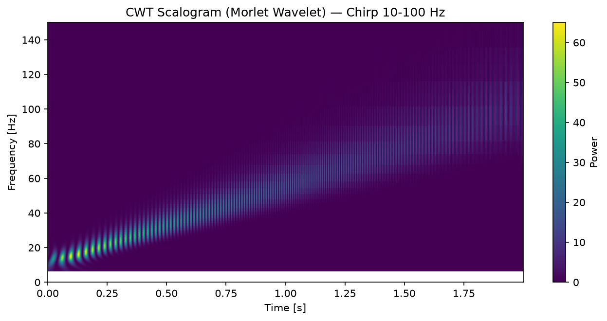
The scalogram clearly shows the frequency increasing from 10 Hz to 100 Hz over time. Compared to an STFT spectrogram, the wavelet scalogram offers higher frequency resolution at low frequencies and higher time resolution at high frequencies, demonstrating the adaptive resolution property.
DWT Example: Multi-Level Decomposition
We perform multi-level DWT decomposition on a noisy signal and visualize the approximation and detail coefficients at each level.
import numpy as np
import matplotlib.pyplot as plt
import pywt

# --- Generate test signal ---
np.random.seed(42)
fs = 500
t = np.arange(0, 1, 1 / fs)
# Low-frequency + high-frequency + noise
clean = np.sin(2 * np.pi * 5 * t) + 0.5 * np.sin(2 * np.pi * 50 * t)
noise = 0.3 * np.random.randn(len(t))
signal = clean + noise

# --- Multi-level DWT decomposition ---
wavelet = "db4"  # Daubechies-4 wavelet
level = 5
coeffs = pywt.wavedec(signal, wavelet, level=level)
# coeffs = [cA5, cD5, cD4, cD3, cD2, cD1]

# --- Visualization ---
fig, axes = plt.subplots(level + 2, 1, figsize=(10, 10), sharex=False)

axes[0].plot(t, signal, "k", linewidth=0.5)
axes[0].set_title("Original Signal")
axes[0].set_ylabel("Amplitude")

axes[1].plot(coeffs[0], "b", linewidth=0.5)
axes[1].set_title(f"Approximation Coefficients (cA{level})")
axes[1].set_ylabel("Amplitude")

for i in range(1, level + 1):
    axes[i + 1].plot(coeffs[i], "r", linewidth=0.5)
    axes[i + 1].set_title(f"Detail Coefficients (cD{level - i + 1})")
    axes[i + 1].set_ylabel("Amplitude")

plt.tight_layout()
plt.show()
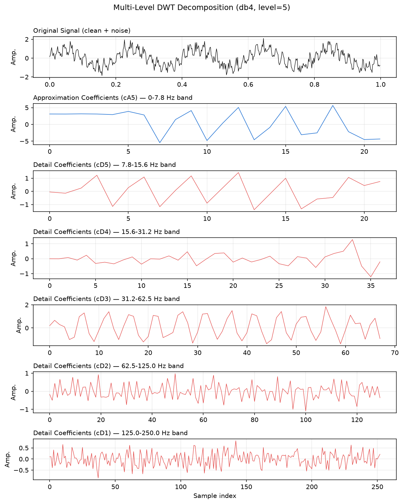
Examining the decomposition results reveals:
- cA5 (approximation coefficients): Contains the lowest-frequency components (the 5 Hz sine wave)
- cD1, cD2 (detail coefficients, high levels): Primarily contain high-frequency noise
- cD3, cD4 (detail coefficients, mid levels): Contain the 50 Hz sine wave component
At sampling frequency \(f_s = 500\,\text{Hz}\) , the detail coefficients at level \(j\) approximately cover the frequency band
\[ \left[\frac{f_s}{2^{j+1}}, \frac{f_s}{2^j}\right] \](the boundaries are not exact since the filters are not ideal brick-wall filters). This gives \(\text{cD}_3\) a band from \(500/16 = 31.25\,\text{Hz}\) to \(500/8 = 62.5\,\text{Hz}\) — exactly where the 50 Hz component lives. The cD3 panel above indeed shows a clean periodic waveform (the 50 Hz sine) dominating that subband. This band placement turns out to be the key to understanding the wavelet-thresholding pitfall discussed below.
Signal Denoising with Wavelet Thresholding
A key application of DWT is wavelet thresholding for signal denoising. Since noise primarily appears in the detail coefficients, zeroing out coefficients below a threshold effectively removes noise.
import numpy as np
import pywt

# --- Generate test signal ---
np.random.seed(42)
fs = 500
t = np.arange(0, 1, 1 / fs)
clean = np.sin(2 * np.pi * 5 * t) + 0.5 * np.sin(2 * np.pi * 50 * t)
noise = 0.3 * np.random.randn(len(t))
signal = clean + noise

# --- DWT decomposition (same level=5 as the MRA example above) ---
wavelet = "db4"
level = 5
coeffs = pywt.wavedec(signal, wavelet, level=level)

# --- Thresholding ---
# Universal threshold (VisuShrink): lambda = sigma * sqrt(2 * log(N))
sigma = np.median(np.abs(coeffs[-1])) / 0.6745  # Robust noise estimation (from cD1)
threshold = sigma * np.sqrt(2 * np.log(len(signal)))

# Apply soft thresholding to detail coefficients
coeffs_thresh = [coeffs[0]]  # Keep approximation coefficients
for c in coeffs[1:]:
    coeffs_thresh.append(pywt.threshold(c, threshold, mode="soft"))

# --- Inverse DWT reconstruction ---
denoised = pywt.waverec(coeffs_thresh, wavelet)

# --- Quantitative evaluation ---
mse_noisy = np.mean((signal - clean) ** 2)
mse_denoised = np.mean((denoised[: len(t)] - clean) ** 2)
print(f"sigma:                  {sigma:.6f}")
print(f"threshold:              {threshold:.6f}")
print(f"MSE of noisy signal:    {mse_noisy:.6f}")
print(f"MSE after denoising:    {mse_denoised:.6f}")
print(f"MSE improvement:        {(1 - mse_denoised / mse_noisy) * 100:.1f}%")
Running this code produces:
sigma:                  0.298703
threshold:              1.053079
MSE of noisy signal:    0.086488
MSE after denoising:    0.133230
MSE improvement:        -54.0%
The improvement is negative — denoising actually made the MSE worse. This is not a coding mistake; it reproduces every time you run this exact PyWavelets code. Sweeping the random seed from 0 to 19 gives a mean improvement of -43.9%, with the best of the 20 runs still at -21.5% — every single trial got worse. We diagnose why below.
Soft thresholding shrinks coefficients exceeding the threshold \(\lambda\) by \(\lambda\) and zeros out those below:
\[\text{soft}(x, \lambda) = \text{sign}(x) \cdot \max(|x| - \lambda, 0) \tag{12}\]The universal threshold \(\lambda = \sigma\sqrt{2 \log N}\) (VisuShrink) is automatically determined from the noise standard deviation \(\sigma\) and signal length \(N\) , requiring no parameter tuning. The noise standard deviation \(\sigma\) is robustly estimated using the MAD (Median Absolute Deviation).
Pitfall: Mismatch Between Decomposition Level and Signal Band
The reason the result above gets worse is that the band used to calibrate the threshold and the bands the threshold is applied to don’t match.
sigmais estimated from the finest-level detail coefficientscoeffs[-1](cD1, the 125-250 Hz band). This band contains essentially no signal energy, only noise, so the \(\sigma\) estimate itself is reasonable.- However, the resulting threshold \(\lambda\) is then applied uniformly to every detail level, cD1 through cD5.
- As the band analysis above showed, cD3 (31.25-62.5 Hz) is dominated by the 50 Hz sine — genuine signal, not noise. Applying a noise-calibrated threshold there means the soft-thresholding shrinkage \(|x| - \lambda\) eats into the signal coefficients themselves, so the signal distortion introduced outweighs the noise removed.
This is a textbook illustration of how VisuShrink’s underlying assumption — “detail coefficients are noise-dominated at every level” — breaks down for signals with narrowband periodic content. The deeper the decomposition, the more likely signal energy spreads across multiple detail bands, making the problem worse.
One fix is to keep the decomposition shallow enough that all of the signal’s dominant frequencies land inside the approximation coefficients (cA). For this signal, both the 5 Hz and 50 Hz components fall inside cA2’s 0-31.25 Hz band at level=2, so shallowing the decomposition to level=2 avoids the collision between the threshold and the signal band.
import numpy as np
import pywt

# --- Generate test signal (identical to above) ---
np.random.seed(42)
fs = 500
t = np.arange(0, 1, 1 / fs)
clean = np.sin(2 * np.pi * 5 * t) + 0.5 * np.sin(2 * np.pi * 50 * t)
noise = 0.3 * np.random.randn(len(t))
signal = clean + noise

# --- DWT decomposition (corrected: level=2) ---
wavelet = "db4"
level = 2
coeffs = pywt.wavedec(signal, wavelet, level=level)

sigma = np.median(np.abs(coeffs[-1])) / 0.6745
threshold = sigma * np.sqrt(2 * np.log(len(signal)))

coeffs_thresh = [coeffs[0]]
for c in coeffs[1:]:
    coeffs_thresh.append(pywt.threshold(c, threshold, mode="soft"))

denoised = pywt.waverec(coeffs_thresh, wavelet)

mse_noisy = np.mean((signal - clean) ** 2)
mse_denoised = np.mean((denoised[: len(t)] - clean) ** 2)
print(f"MSE of noisy signal:    {mse_noisy:.6f}")
print(f"MSE after denoising:    {mse_denoised:.6f}")
print(f"MSE improvement:        {(1 - mse_denoised / mse_noisy) * 100:.1f}%")
This produces:
MSE of noisy signal:    0.086488
MSE after denoising:    0.049084
MSE improvement:        43.2%
Just changing the decomposition level from 5 to 2 turns a -54.0% result into +43.2%. Note that \(\sigma\)
and \(\lambda\)
themselves are unchanged (cD1 is identical regardless of level) — what changed is that the threshold is now only applied to detail bands that are genuinely noise-dominated (cD1: 125-250 Hz, cD2: 62.5-125 Hz).
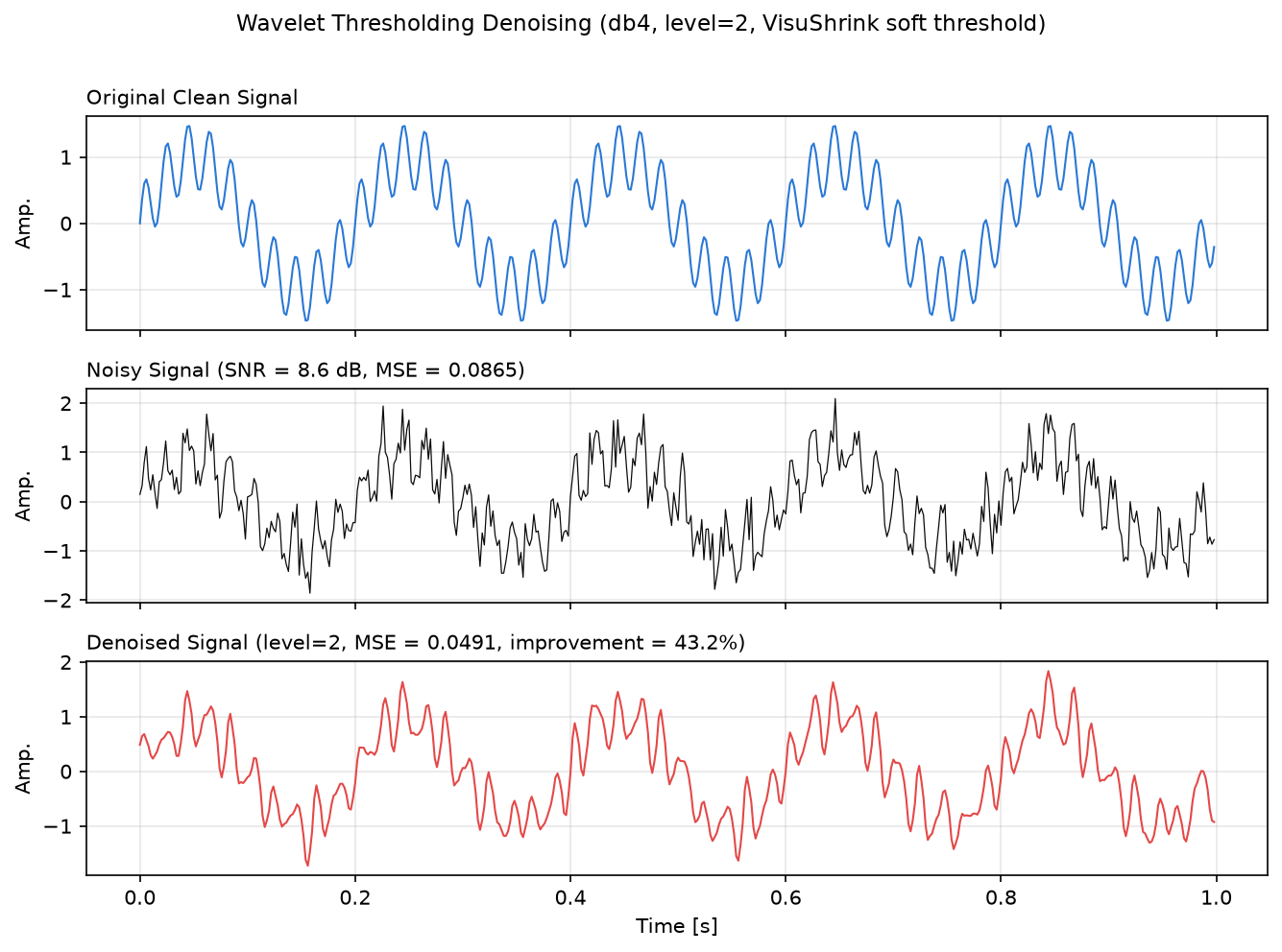
This is a practical lesson: the decomposition level in wavelet denoising is a hyperparameter, and you should verify that the signal’s frequency content is consistent with the bands used to calibrate the threshold before trusting the result. pywt.wavedec will happily compute the maximum level supported by the signal length by default, but blindly using that maximum can produce exactly this kind of degradation.
Comparison: FFT vs STFT vs Wavelet
| Feature | FFT | STFT | Wavelet |
|---|---|---|---|
| Time resolution | None | Fixed | Adaptive (high at high-freq) |
| Frequency resolution | High (global) | Fixed | Adaptive (high at low-freq) |
| Basis function | Sinusoid | Windowed sinusoid | Mother wavelet |
| Output | 1D spectrum | 2D (time-frequency) | 2D (time-scale) |
| Inverse transform | Yes | Yes | Yes |
| Complexity | \(O(N \log N)\) | \(O(N L \log L)\) | CWT: \(O(NS)\) , DWT: \(O(N)\) |
| Primary use | Stationary signals | Speech/music analysis | Non-stationary, denoising |
Here \(L\) is the STFT window length and \(S\) is the number of CWT scales. DWT achieves \(O(N)\) complexity through its filter bank implementation, making it highly efficient.
Guidelines for choosing the appropriate method:
- Stationary signals where you need the overall frequency content -> FFT
- Time-varying frequencies tracked at uniform resolution -> STFT
- Simultaneous detection of slow trends and rapid transients -> Wavelet Transform
Recent Developments: Deep Learning Time Series Forecasting
Wavelet transforms are not confined to classical signal processing — they are actively studied today as a preprocessing and feature-extraction layer inside deep learning time series forecasters.
Zhou et al. (2025), “ Multi-Order Wavelet Derivative Transform for Deep Time Series Forecasting ” (arXiv:2505.11781), proposes the Wavelet Derivative Transform (WDT), which applies the wavelet transform not to the raw signal but to its derivative. Where Fourier-based methods struggle to capture time-sensitive multi-scale patterns, WDT emphasizes the rate of change, making abrupt fluctuations easier to detect. The transform is embedded in a framework called WaveTS, which decomposes and refines the input series into multi-scale time-frequency coefficients and then reconstructs the time domain via the inverse transform. Across 10 benchmark datasets, it reportedly achieves state-of-the-art forecasting accuracy while retaining high computational efficiency. It’s a striking example of the MRA band-splitting idea covered in this article being applied directly to input representation design for Transformer-based forecasters.
Summary
This article covered the mathematical foundations and Python implementations of the wavelet transform.
- CWT varies scale and translation continuously, achieving adaptive time-frequency resolution
- DWT achieves efficient \(O(N)\) decomposition through dyadic sampling and filter banks
- Wavelet thresholding is a practical denoising technique that applies thresholds to detail coefficients, but if the decomposition level doesn’t match the signal’s frequency content, it can make the MSE worse rather than better (measured: -54.0% at level=5, +43.2% once corrected to level=2) — always verify that the band used to calibrate the threshold matches the bands it’s applied to
- FFT, STFT, and wavelet transforms each excel in different scenarios; choosing the right tool depends on the analysis target
The wavelet transform extends beyond signal processing into image compression (JPEG 2000), financial data analysis, biomedical signal processing, seismic analysis, and many other fields.
Related Articles
- Fast Fourier Transform (FFT): Theory and Python Implementation - Detailed coverage of the Fourier transform, providing the foundation for comparison with wavelets.
- DTFT vs DFT vs FFT: Definitions, Relationships, and Python Implementation - Clarifies the hierarchy “continuous-frequency representation of a discrete signal (DTFT) → its finite-frequency-sampled version (DFT)” that underlies wavelet analysis.
- Window Functions and Power Spectral Density (PSD): Theory and Python Implementation - FFT window functions and PSD estimation in detail.
- Autocorrelation Function: Theory and Python Implementation - The autocorrelation framework (the Fourier pair of the PSD) is the natural lens for the within-scale and across-scale structure of wavelet coefficients.
- Low-Pass Filter Design and Comparison - Enables comparison between classical filter design and the wavelet approach.
- Time-Series Anomaly Detection: From Statistical Methods to Kalman Filter in Python - Anomaly detection methods where wavelet transform can serve as preprocessing.
- Wiener Filter: Optimal Linear Filtering Theory and Python Implementation - A different approach to optimal noise removal.
- Frequency Characteristics of the Exponential Moving Average (EMA) Filter - Helps understand the difference between time-domain filtering and wavelet-based frequency separation.
- Moving Average Filters Compared: SMA, WMA, and EMA in Python - Helps understand the relationship between time-domain filters and wavelet filter banks.
- Matplotlib Practical Tips: Creating Publication-Quality Figures - Tips for producing higher-quality scalogram visualizations.
- Short-Time Fourier Transform (STFT): Theory and Python Implementation - Fixed-window time-frequency analysis; the canonical comparison target that wavelet’s variable window overcomes.
- Wavelet Packet Transform and Best Basis Selection - Extension of DWT that recursively splits the high-frequency branch as well, with signal-adaptive best-basis selection.
- Hilbert Transform and the Analytic Signal: Theory and Python Implementation - Hilbert-Huang Transform (HHT) is a frequent point of comparison for non-stationary signal analysis.
- Bandpass Filter Design and Python Implementation - Classical IIR band separation that relates to the filter-bank interpretation of DWT.
- Time-Frequency Analysis Guide - Integrated hub that places wavelets alongside FFT, STFT, and the Hilbert transform with a use-case decision flow built on time-frequency resolution trade-offs.
References
- Mallat, S. (2008). A Wavelet Tour of Signal Processing: The Sparse Way (3rd ed.). Academic Press.
- Daubechies, I. (1992). Ten Lectures on Wavelets. SIAM.
- Zhou, Z., Hu, J., Wen, Q., Kwok, J. T., & Liang, Y. (2025). Multi-Order Wavelet Derivative Transform for Deep Time Series Forecasting . arXiv:2505.11781.
- PyWavelets documentation
- SciPy Signal Processing documentation