Introduction
In the FFT article , we covered the DFT algorithm and basic frequency analysis. We briefly touched on using the Hann window to mitigate spectral leakage, but there are many types of window functions, and choosing the right one for the task at hand is essential.
Moreover, the amplitude spectrum from FFT shows “how much amplitude exists at each frequency,” but in practice we often need to know the signal power per unit frequency. This quantity is the Power Spectral Density (PSD).
This article dives deeper into the mathematics behind spectral leakage, compares the characteristics of major window functions, and implements PSD estimation via Welch’s method in Python.
Mathematical Understanding of Spectral Leakage
Finite-Length Signals and the Rectangular Window
In practice, we can never record a signal for infinite duration. We acquire a finite-length signal \(x[n]\) (\(n = 0, 1, \ldots, N-1\) ). Mathematically, this is equivalent to multiplying an infinite-length signal \(x_\infty[n]\) by a rectangular window \(w_R[n]\) .
\[x[n] = x_\infty[n] \cdot w_R[n] \tag{1}\]The rectangular window is defined as:
\[w_R[n] = \begin{cases} 1, & 0 \leq n \leq N-1 \\ 0, & \text{otherwise} \end{cases} \tag{2}\]Effect in the Frequency Domain
Multiplication in the time domain corresponds to convolution in the frequency domain.
\[X(f) = X_\infty(f) * W_R(f) \tag{3}\]The Fourier transform of the rectangular window is the Dirichlet kernel, which in continuous approximation is proportional to the sinc function.
\[W_R(f) \approx N \cdot \text{sinc}(Nf) \cdot e^{-j\pi f(N-1)} \tag{4}\]This sinc function has a broad mainlobe and slowly decaying sidelobes. Through the convolution in Eq. \((3)\) , a spectrum that should be concentrated at a single frequency spreads to adjacent frequencies via these sidelobes. This is the mathematical origin of spectral leakage.
Mainlobe and Sidelobes
The frequency characteristics of a window function are described by two key elements:
- Mainlobe: The primary peak around the center frequency. A narrower mainlobe yields higher frequency resolution.
- Sidelobes: Secondary peaks on either side of the mainlobe. Lower sidelobe levels mean less spectral leakage.
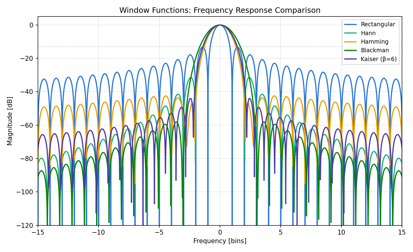
The rectangular window has a peak sidelobe level of only \(-13\) dB, which means weak signal components near a strong tone can be buried under the sidelobes. By choosing different window functions, we can control this tradeoff.
Major Window Functions
Below are the mathematical definitions of commonly used window functions, all of length \(N\) .
Rectangular Window
\[w[n] = 1, \quad 0 \leq n \leq N-1 \tag{5}\]Equivalent to applying no window. It has the narrowest mainlobe and therefore the best frequency resolution, but the sidelobes are large and spectral leakage is severe.
Hann Window
\[w[n] = 0.5\left(1 - \cos\left(\frac{2\pi n}{N-1}\right)\right) \tag{6}\]A cosine-based window that tapers to zero at both ends. The sidelobe decay rate of \(-18\) dB/oct is fast, making it the most widely used general-purpose window.
Hamming Window
\[w[n] = 0.54 - 0.46\cos\left(\frac{2\pi n}{N-1}\right) \tag{7}\]Similar to the Hann window, but the endpoints do not reach zero (they have a value of approximately 0.08). The first sidelobe is suppressed to \(-43\) dB, but the far sidelobe decay is only \(-6\) dB/oct, slower than the Hann window.
Blackman Window
\[w[n] = 0.42 - 0.5\cos\left(\frac{2\pi n}{N-1}\right) + 0.08\cos\left(\frac{4\pi n}{N-1}\right) \tag{8}\]Composed of three cosine terms. The first sidelobe is extremely low at \(-58\) dB, making it suitable for high dynamic range analysis, but the wider mainlobe reduces frequency resolution.
Kaiser Window
\[w[n] = \frac{I_0\left(\beta\sqrt{1 - \left(\frac{2n}{N-1} - 1\right)^2}\right)}{I_0(\beta)} \tag{9}\]Here \(I_0\) is the zeroth-order modified Bessel function of the first kind, and \(\beta\) is the shape parameter. By adjusting \(\beta\) , you can continuously control the tradeoff between mainlobe width and sidelobe suppression. \(\beta = 0\) gives the rectangular window, and \(\beta \approx 5.4\) approximates the Hamming window.
Window Function Characteristics Comparison
| Window | Mainlobe Width | Peak Sidelobe [dB] | Sidelobe Decay | ENBW (bins) |
|---|---|---|---|---|
| Rectangular | 2 bins | -13 | -6 dB/oct | 1.00 |
| Hann | 4 bins | -32 | -18 dB/oct | 1.50 |
| Hamming | 4 bins | -43 | -6 dB/oct | 1.36 |
| Blackman | 6 bins | -58 | -18 dB/oct | 1.73 |
| Kaiser (β=6) | Variable | Variable | Variable | Variable |
ENBW (Equivalent Noise Bandwidth) indicates how many frequency bins of bandwidth a window effectively has for white noise. A larger value means more noise influence on the estimate.
Deriving ENBW
ENBW quantifies “how many bins wide an equivalent rectangular filter would need to be to pass the same white-noise power as the windowed periodogram’s peak gain.” Here is the derivation.
Let \(W[k]\) be the DFT of a window \(w[n]\) (\(n = 0, \ldots, N-1\) ). By Parseval’s theorem, the sum of power in the frequency domain equals \(N\) times the sum of power in the time domain.
\( \sum_{k=0}^{N-1} |W[k]|^2 = N \sum_{n=0}^{N-1} w[n]^2 \tag{15} \)
The peak power gain of the frequency response, at \(k=0\) (DC), is \(|W[0]|^2 = \left(\sum_n w[n]\right)^2\) . ENBW (in bins) is defined so that “peak power gain × ENBW” equals the total power in Eq. \((15)\) .
\[\text{ENBW} \cdot \left(\sum_{n=0}^{N-1} w[n]\right)^2 = N \sum_{n=0}^{N-1} w[n]^2 \tag{16}\]Solving for ENBW gives:
\( \text{ENBW} = N \cdot \dfrac{\sum_{n=0}^{N-1} w[n]^2}{\left(\sum_{n=0}^{N-1} w[n]\right)^2} \tag{17} \)
For the rectangular window (\(w[n]=1\) ), the numerator is \(N \cdot N = N^2\) and the denominator is \(N^2\) , so \(\text{ENBW}=1\) . We verify Eq. \((17)\) numerically in Python.
import numpy as np
from scipy.signal.windows import hann, hamming, blackman, kaiser

def enbw(w):
    """Eq. (17): equivalent noise bandwidth of a window, in bins"""
    N = len(w)
    return N * np.sum(w**2) / np.sum(w)**2

N = 1024
windows = {
    'Rectangular': np.ones(N),
    'Hann': hann(N),
    'Hamming': hamming(N),
    'Blackman': blackman(N),
    'Kaiser (β=6)': kaiser(N, beta=6),
}
for name, w in windows.items():
    print(f"{name:15s} ENBW = {enbw(w):.4f} bins")
Actual output:
Rectangular     ENBW = 1.0000 bins
Hann            ENBW = 1.5015 bins
Hamming         ENBW = 1.3638 bins
Blackman        ENBW = 1.7284 bins
Kaiser (β=6)    ENBW = 1.4682 bins
These numerically computed values match the approximate figures in the table above (Rectangular 1.00, Hann 1.50, Hamming 1.36, Blackman 1.73).
Window Functions: Frequency Response Comparison (Python)
Let us generate all window functions and compare their frequency responses on a dB scale.
import numpy as np
import matplotlib.pyplot as plt
from scipy.signal.windows import hann, hamming, blackman, kaiser

# Window length
N = 64
# FFT size (zero-padded for interpolation)
N_fft = 4096

# Generate each window function
windows = {
    'Rectangular': np.ones(N),
    'Hann': hann(N),
    'Hamming': hamming(N),
    'Blackman': blackman(N),
    'Kaiser (β=6)': kaiser(N, beta=6),
}

# Compute and plot frequency responses
fig, ax = plt.subplots(figsize=(10, 6))

for name, w in windows.items():
    # Compute frequency response via FFT
    W = np.fft.fft(w, n=N_fft)
    W_shift = np.fft.fftshift(W)
    # Normalize (mainlobe peak at 0 dB)
    W_dB = 20 * np.log10(np.maximum(np.abs(W_shift) / np.abs(W_shift).max(), 1e-12))
    # Frequency axis (in bins)
    freq_bins = np.linspace(-N / 2, N / 2, N_fft)
    ax.plot(freq_bins, W_dB, label=name)

ax.set_xlim(-15, 15)
ax.set_ylim(-120, 5)
ax.set_xlabel('Frequency [bins]')
ax.set_ylabel('Magnitude [dB]')
ax.set_title('Window Functions: Frequency Response Comparison')
ax.legend()
ax.grid(True, alpha=0.3)
plt.tight_layout()
plt.show()
This plot visually confirms that the rectangular window has the narrowest mainlobe but the largest sidelobes, while the Blackman window has very low sidelobes at the cost of a wider mainlobe.
Power Spectral Density (PSD)
Definition and Physical Meaning
The amplitude spectrum \(|X[k]|\) shows the signal amplitude at each frequency bin, but it depends on the FFT length \(N\) and sampling rate \(f_s\) , making direct comparison between spectra obtained under different conditions difficult.
Power Spectral Density (PSD) is defined as signal power per unit frequency and shows how a signal’s power is distributed across the frequency axis. Its unit is \(\text{V}^2/\text{Hz}\) (or the appropriate physical unit squared per Hz).
An important property of PSD is that integrating it over all frequencies yields the total signal power (variance).
\[\int_0^{f_s/2} S_{xx}(f) \, df = \sigma_x^2 \tag{10}\]Difference from Amplitude Spectrum
| Property | Amplitude Spectrum | Power Spectral Density |
|---|---|---|
| Value | \(\|X[k]\|\) | \(S_{xx}(f)\) |
| Unit | V (signal unit) | \(\text{V}^2/\text{Hz}\) |
| N dependency | Proportional to N | Independent of N |
| Use case | Check amplitude at a frequency | Quantitative power distribution |
PSD Estimation Methods
Periodogram
The simplest PSD estimator is the periodogram, computed directly from the FFT result.
\[\hat{S}_{xx}[k] = \frac{|X[k]|^2}{N \cdot f_s \cdot U} \tag{11}\]Here \(X[k]\) is the DFT of the windowed signal and \(U = \frac{1}{N}\sum_{n=0}^{N-1} w[n]^2\) is the window power correction factor (\(U=1\) for the rectangular window). The periodogram is asymptotically unbiased (unbiased as \(N \to \infty\) ), but suffers from high variance. Even increasing the data length \(N\) does not reduce the variance, so the estimate fluctuates significantly due to noise.
Numerically Verifying That Periodogram Variance Does Not Decrease
The claim that “variance does not decrease even as \(N\) grows” is counter-intuitive, so let’s verify it directly: generate unit-variance white noise repeatedly, compute the periodogram each time, and measure the spread (coefficient of variation = std/mean) of the estimate at a fixed frequency bin. For comparison, we compute the same coefficient of variation for Welch’s method on the same data.
import numpy as np
from scipy.signal import welch

fs = 1000.0
n_trials = 200

def periodogram_cv(N, trials=n_trials, seed=0):
    """Compute the periodogram of N-point white noise `trials` times and
    return the coefficient of variation (std/mean) at a fixed bin"""
    rng = np.random.default_rng(seed)
    vals = []
    for _ in range(trials):
        x = rng.standard_normal(N)
        X = np.fft.rfft(x)
        psd = (np.abs(X)**2) / (N * fs)
        psd[1:-1] *= 2
        idx = max(1, N // 8)  # a fixed bin away from DC/Nyquist
        vals.append(psd[idx])
    vals = np.array(vals)
    return vals.mean(), vals.std() / vals.mean()

for N in [256, 1024, 4096, 16384]:
    mean, cv = periodogram_cv(N)
    print(f"N={N:6d}  periodogram mean={mean:.6f}  CV(std/mean)={cv:.3f}")

def welch_cv(N, nperseg, trials=n_trials, seed=1):
    rng = np.random.default_rng(seed)
    vals = []
    for _ in range(trials):
        x = rng.standard_normal(N)
        f, p = welch(x, fs=fs, window='hann', nperseg=nperseg, noverlap=nperseg // 2)
        idx = max(1, len(f) // 8)
        vals.append(p[idx])
    vals = np.array(vals)
    K = (N - nperseg) // (nperseg // 2) + 1  # number of segments averaged
    return vals.mean(), vals.std() / vals.mean(), K

print()
for nperseg in [256, 128, 64]:
    mean, cv, K = welch_cv(16384, nperseg)
    print(f"Welch nperseg={nperseg:4d} (K={K:3d}segs)  mean={mean:.6f}  CV(std/mean)={cv:.3f}  1/sqrt(K)={1/np.sqrt(K):.3f}")
Actual output:
N=   256  periodogram mean=0.002234  CV(std/mean)=1.041
N=  1024  periodogram mean=0.001887  CV(std/mean)=1.023
N=  4096  periodogram mean=0.002017  CV(std/mean)=1.160
N= 16384  periodogram mean=0.002157  CV(std/mean)=0.983

Welch nperseg= 256 (K=127segs)  mean=0.002005  CV(std/mean)=0.084  1/sqrt(K)=0.089
Welch nperseg= 128 (K=255segs)  mean=0.002011  CV(std/mean)=0.068  1/sqrt(K)=0.063
Welch nperseg=  64 (K=511segs)  mean=0.002005  CV(std/mean)=0.047  1/sqrt(K)=0.044
The periodogram’s coefficient of variation stays at roughly 1.0 even as \(N\) grows 64-fold from 256 to 16384, confirming that variance does not decrease with data length (this follows from the periodogram’s estimate being approximately chi-squared distributed with 2 degrees of freedom, whose relative standard deviation approaches 1 independent of \(N\) ). Welch’s method, by contrast, sees its coefficient of variation drop to 0.084, 0.068, and 0.047 as the segment count \(K\) rises to 127, 255, and 511 — closely matching the theoretical \(1/\sqrt{K}\) values of 0.089, 0.063, and 0.044. This is a direct consequence of the central-limit-theorem property that averaging \(K\) independent (or near-independent) estimates reduces variance by a factor of \(1/K\) , and it quantitatively confirms the mechanism by which Welch’s method reduces variance.
Welch’s Method
Welch’s method (1967) is a practical technique for reducing periodogram variance. The procedure is:
- Divide the signal into segments of length \(L\) with overlap
- Apply a window function \(w[n]\) to each segment
- Compute the modified periodogram for each segment
- Average all segment results
The modified periodogram of the \(i\) -th segment is defined as:
\[\hat{S}_{xx}^{(i)}[k] = \frac{1}{L \cdot f_s \cdot U} \left| \sum_{n=0}^{L-1} x_i[n] \cdot w[n] \cdot e^{-j2\pi kn/L} \right|^2 \tag{12}\]where \(U\) is the window power normalization factor:
\[U = \frac{1}{L}\sum_{n=0}^{L-1} w[n]^2 \tag{13}\]Averaging over \(K\) segments gives the Welch PSD estimate:
\[\hat{S}_{xx}^{\text{Welch}}[k] = \frac{1}{K}\sum_{i=1}^{K} \hat{S}_{xx}^{(i)}[k] \tag{14}\]Overlap is used to make effective use of the data and increase the number of segments available for averaging. A 50% overlap is typical. Excessive overlap increases inter-segment correlation and diminishes the averaging benefit.
Segment length tradeoff: longer segments improve frequency resolution but yield fewer segments for averaging (higher variance). Shorter segments reduce variance but degrade frequency resolution (and if the true PSD varies within a bin, shorter segments also introduce more smoothing bias).
This bias-variance tradeoff had been a long-standing practical issue. Astfalck, Sykulski, and Cripps (2023), “Debiasing Welch’s Method for Spectral Density Estimation” ( arXiv:2312.13643 , accepted in Biometrika), propose a debiasing technique that reduces finite-sample bias while preserving Welch’s method’s computational complexity and asymptotic consistency. The paper also shows that evaluating segments on an irregularly spaced frequency grid can achieve additional variance reduction, with implementations released in both Python and R. Where the classic tradeoff says “shorter segments mean less variance but more bias,” this is a 2023-and-later research direction that actively corrects the bias side of that tradeoff.
Practical PSD Estimation in Python
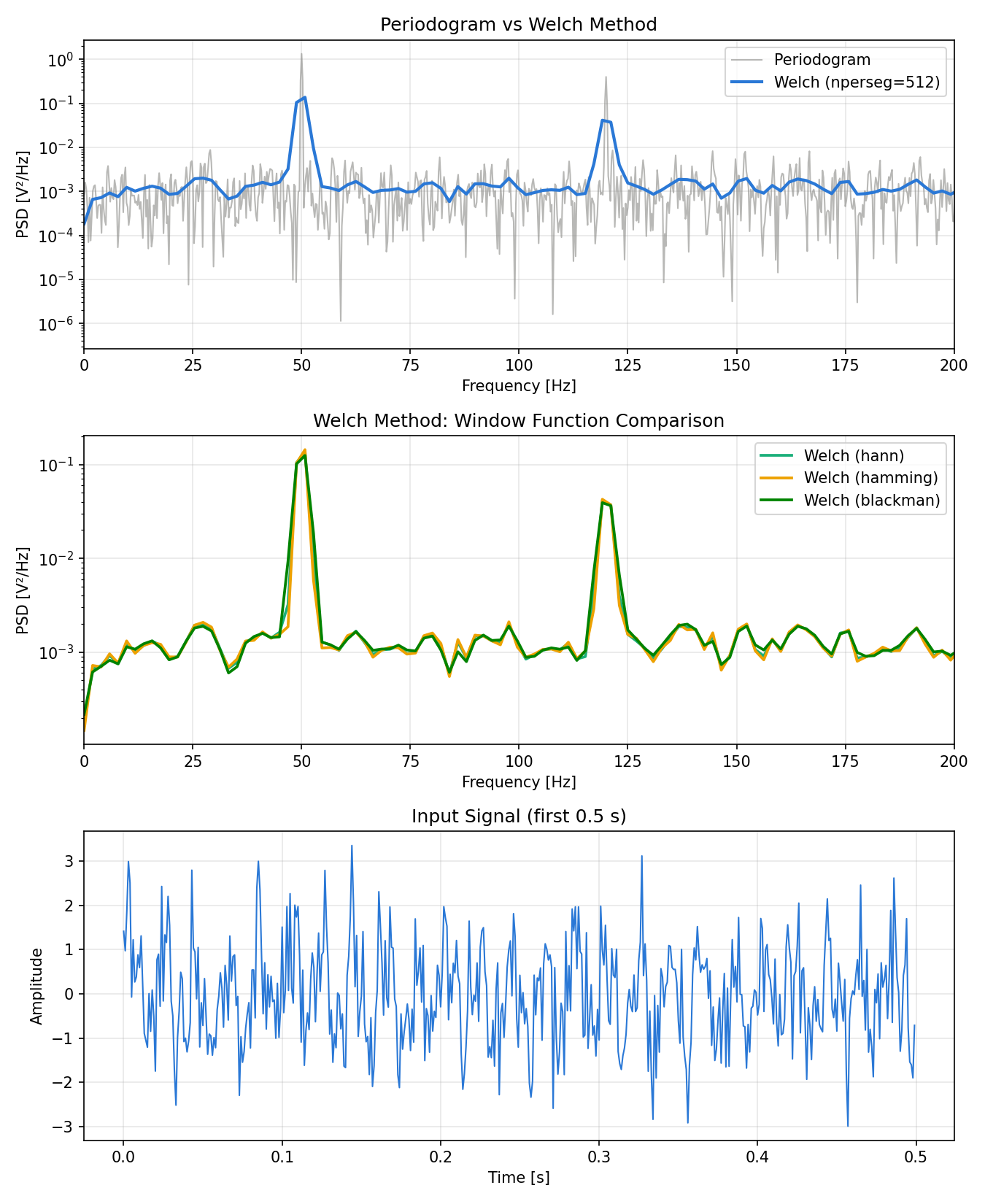
We generate a test signal with two sinusoids (50 Hz and 120 Hz) plus white noise, then compare PSD estimates from the periodogram and Welch’s method.
import numpy as np
import matplotlib.pyplot as plt
from scipy.signal import welch
from scipy.signal.windows import hann

# --- Generate test signal ---
np.random.seed(0)
fs = 1000            # Sampling frequency [Hz]
T = 4.0              # Signal duration [s]
t = np.arange(0, T, 1/fs)
N_total = len(t)

# 50 Hz (amplitude 1.0) and 120 Hz (amplitude 0.5) + white noise
signal = (np.sin(2 * np.pi * 50 * t)
          + 0.5 * np.sin(2 * np.pi * 120 * t)
          + 0.8 * np.random.randn(N_total))

# --- 1. Periodogram (manual implementation) ---
window = hann(N_total)
X = np.fft.fft(signal * window)
freqs_periodo = np.fft.fftfreq(N_total, 1/fs)
# Window power correction
U = np.mean(window**2)
# One-sided periodogram
psd_periodo = (np.abs(X[:N_total//2])**2) / (N_total * fs * U)
psd_periodo[1:-1] *= 2  # Double all bins except DC and Nyquist
freqs_periodo = freqs_periodo[:N_total//2]

# --- 2. Welch's method (scipy.signal.welch) ---
freqs_welch, psd_welch = welch(signal, fs=fs, window='hann',
                                nperseg=512, noverlap=256)

# --- 3. Window function comparison ---
windows_list = ['hann', 'hamming', 'blackman']
psd_results = {}
for win_name in windows_list:
    f, p = welch(signal, fs=fs, window=win_name,
                 nperseg=512, noverlap=256)
    psd_results[win_name] = (f, p)

# --- Plot ---
fig, axes = plt.subplots(3, 1, figsize=(10, 12))

# (a) Periodogram vs Welch's method
axes[0].semilogy(freqs_periodo, psd_periodo, alpha=0.5, label='Periodogram')
axes[0].semilogy(freqs_welch, psd_welch, label='Welch (nperseg=512)')
axes[0].set_xlabel('Frequency [Hz]')
axes[0].set_ylabel('PSD [V²/Hz]')
axes[0].set_title('Periodogram vs Welch Method')
axes[0].legend()
axes[0].set_xlim(0, 200)
axes[0].grid(True, alpha=0.3)

# (b) Welch's method with different windows
for win_name, (f, p) in psd_results.items():
    axes[1].semilogy(f, p, label=f'Welch ({win_name})')
axes[1].set_xlabel('Frequency [Hz]')
axes[1].set_ylabel('PSD [V²/Hz]')
axes[1].set_title('Welch Method: Window Function Comparison')
axes[1].legend()
axes[1].set_xlim(0, 200)
axes[1].grid(True, alpha=0.3)

# (c) Input signal waveform
axes[2].plot(t[:500], signal[:500])
axes[2].set_xlabel('Time [s]')
axes[2].set_ylabel('Amplitude')
axes[2].set_title('Input Signal (first 0.5 s)')
axes[2].grid(True, alpha=0.3)

plt.tight_layout()
plt.show()
Continuing directly from the code above, let’s check the actual PSD values at the peak frequencies and the fluctuation of the noise floor.
# --- Check peak values ---
idx_w50 = np.argmin(np.abs(freqs_welch - 50))
idx_w120 = np.argmin(np.abs(freqs_welch - 120))
print("=== Welch's method (nperseg=512, noverlap=256) ===")
print(f"Near 50Hz: freq={freqs_welch[idx_w50]:.2f} Hz, PSD={psd_welch[idx_w50]:.5f} V^2/Hz")
print(f"Near 120Hz: freq={freqs_welch[idx_w120]:.2f} Hz, PSD={psd_welch[idx_w120]:.5f} V^2/Hz")
print(f"Peak ratio (120Hz/50Hz) = {psd_welch[idx_w120] / psd_welch[idx_w50]:.4f} (theory 0.5^2=0.25)")

idx_p50 = np.argmin(np.abs(freqs_periodo - 50))
idx_p120 = np.argmin(np.abs(freqs_periodo - 120))
print()
print("=== Periodogram ===")
print(f"Near 50Hz: freq={freqs_periodo[idx_p50]:.2f} Hz, PSD={psd_periodo[idx_p50]:.5f} V^2/Hz")
print(f"Near 120Hz: freq={freqs_periodo[idx_p120]:.2f} Hz, PSD={psd_periodo[idx_p120]:.5f} V^2/Hz")
print(f"Peak ratio (120Hz/50Hz) = {psd_periodo[idx_p120] / psd_periodo[idx_p50]:.4f}")

# --- Coefficient of variation of the noise floor (130-200 Hz band) ---
mask_p = (freqs_periodo > 130) & (freqs_periodo < 200)
mask_w = (freqs_welch > 130) & (freqs_welch < 200)
print()
print(f"Noise floor CV (130-200Hz) Periodogram: {psd_periodo[mask_p].std() / psd_periodo[mask_p].mean():.3f}")
print(f"Noise floor CV (130-200Hz) Welch:       {psd_welch[mask_w].std() / psd_welch[mask_w].mean():.3f}")
Actual output:
=== Welch's method (nperseg=512, noverlap=256) ===
Near 50Hz: freq=50.78 Hz, PSD=0.13720 V^2/Hz
Near 120Hz: freq=119.14 Hz, PSD=0.04132 V^2/Hz
Peak ratio (120Hz/50Hz) = 0.3012 (theory 0.5^2=0.25)

=== Periodogram ===
Near 50Hz: freq=50.00 Hz, PSD=1.33429 V^2/Hz
Near 120Hz: freq=120.00 Hz, PSD=0.40055 V^2/Hz
Peak ratio (120Hz/50Hz) = 0.3002

Noise floor CV (130-200Hz) Periodogram: 1.099
Noise floor CV (130-200Hz) Welch:       0.289
The periodogram shows large fluctuations in the estimate, whereas Welch’s method produces a much smoother result through averaging. The peaks at 50 Hz and 120 Hz are clearly visible, and both methods give a peak ratio around 0.30, close to the theoretical value for an amplitude ratio of 0.5 (\(0.5^2=0.25\) ) — the small deviation comes from finite frequency resolution and residual noise. Comparing the coefficient of variation (std/mean) of the noise floor, the periodogram sits at 1.099 (close to the theoretical ~1.0, reflecting its high variance), while Welch’s method drops to 0.289 — close to the theoretical \(1/\sqrt{14} \approx 0.267\) for the \(K=14\) segments used here (computed from \(N_{\text{total}}=4000\) , nperseg=512, noverlap=256).
Practical Pitfall: Scalloping Loss and the Picket-Fence Effect
Even after applying a window, if the signal’s frequency does not align exactly with an FFT bin, the estimated amplitude/power is underestimated. This is known as the “picket-fence effect,” and the resulting loss is called scalloping loss.
A window’s frequency response \(W(f)\) reaches its maximum at \(f=0\) (bin center) and its minimum exactly halfway between two bins (a 0.5-bin offset). Scalloping loss (in dB) is defined as:
\[L_{\text{scallop}} = 20 \log_{10} \frac{|W(0.5)|}{|W(0)|} \tag{18}\]We compute the estimated amplitude for a signal exactly on a 40 Hz bin versus one offset by 0.5 bin (around 40.5 Hz), for the rectangular, Hann, and flat-top windows.
import numpy as np
from scipy.signal import get_window
from scipy.signal.windows import hann

N = 256
fs = 256.0
n = np.arange(N)

def peak_amplitude(freq, window):
    """Windows a freq[Hz] sinusoid and estimates the FFT peak amplitude,
    corrected for the window's coherent gain"""
    x = np.sin(2 * np.pi * freq / fs * n)
    X = np.fft.rfft(x * window)
    mag = np.abs(X) / (np.sum(window) / 2)
    return mag.max()

w_rect = np.ones(N)
w_hann = hann(N, sym=False)
w_flattop = get_window('flattop', N, fftbins=True)

for name, w in [('Rectangular', w_rect), ('Hann', w_hann), ('Flattop', w_flattop)]:
    on_bin = peak_amplitude(40.0, w)     # exactly on a bin
    off_bin = peak_amplitude(40.5, w)    # offset by 0.5 bin
    loss_db = 20 * np.log10(off_bin / on_bin)
    print(f"{name:12s} on-bin={on_bin:.4f}  off-bin={off_bin:.4f}  scalloping loss={loss_db:.3f} dB")

# ENBW of the flat-top window (recomputed at N=1024)
N2 = 1024
w_flattop_1024 = get_window('flattop', N2, fftbins=True)
enbw_flattop = N2 * np.sum(w_flattop_1024**2) / np.sum(w_flattop_1024)**2
print(f"\nFlattop ENBW (N={N2}) = {enbw_flattop:.4f} bins")
Actual output:
Rectangular  on-bin=1.0000  off-bin=0.6392  scalloping loss=-3.887 dB
Hann         on-bin=1.0000  off-bin=0.8488  scalloping loss=-1.424 dB
Flattop      on-bin=1.0000  off-bin=0.9989  scalloping loss=-0.010 dB

Flattop ENBW (N=1024) = 3.7702 bins
The rectangular window underestimates the amplitude by up to about 3.9 dB (roughly 36% in amplitude), while the Hann window keeps the loss to about 1.4 dB, and the flat-top window brings it down to a negligible 0.010 dB. This is because the flat-top window is designed to have a flat mainlobe, and can be generated with scipy.signal.get_window('flattop', N). The tradeoff is a much wider mainlobe (ENBW): the flat-top window’s ENBW is about 3.77 bins, 2.5 times that of the Hann window (1.50 bins). In short, the flat-top window is ideal for accurately measuring the absolute amplitude of a single tone (e.g., calibration), at a significant cost to the ability to resolve closely spaced frequencies.
Note that scipy.signal.get_window(name, N) provides a unified interface that accepts parameterized windows as strings or tuples, such as 'hann' or ('kaiser', 6.0), and can be passed directly to the window argument of scipy.signal.welch. In practice, a convenient workflow is to prototype the desired window with get_window and pass it straight to welch.
Two practical mitigations for this effect are:
- Zero-padding interpolation: increasing the FFT size raises the chance of landing closer to the true peak, but it does not change the actual frequency resolution (ENBW) — it is only a cosmetic interpolation.
- Window selection: use the flat-top window when absolute amplitude accuracy matters, and a window close to rectangular (e.g., Hann) when frequency resolution matters.
Window Function Selection Guidelines
| Use Case | Recommended Window | Reason |
|---|---|---|
| General-purpose analysis | Hann | Good balance of sidelobe suppression and resolution |
| Resolving close frequencies | Rectangular / Kaiser (low β) | Narrowest mainlobe |
| High dynamic range analysis | Blackman / Kaiser (high β) | Lowest sidelobes for detecting weak signals |
| Hardware / real-time | Hamming | Simple computation, non-zero at endpoints |
In practice, it is recommended to start with the Hann window and switch to other windows as needed.
Summary
- Spectral leakage occurs because finite-length signal truncation (rectangular windowing) causes convolution in the frequency domain
- Window functions control the tradeoff between mainlobe width and sidelobe suppression; options include Hann, Hamming, Blackman, and Kaiser for different purposes
- Power Spectral Density (PSD) expresses power per unit frequency, enabling comparison across different measurement conditions
- The periodogram has high variance, so Welch’s method with segment averaging is the standard practical estimator
- Window function selection also affects PSD estimation quality, so choosing appropriately for the analysis objective is important
Related Articles
- DTFT vs DFT vs FFT: Definitions, Relationships, and Python Implementation - Lays out the three-level hierarchy that underpins this article’s finite-length DFT and spectral-leakage discussion.
- Fast Fourier Transform (FFT): Algorithm and Python Implementation - Covers the DFT/FFT algorithms and basic frequency analysis that serve as prerequisites for this article.
- Notch Filter Design and Python Implementation - IIR filter design for surgically removing a specific frequency (e.g. power-line hum) identified from the PSD.
- Frequency Characteristics of the Exponential Moving Average (EMA) Filter - A reference for understanding filter frequency response concepts.
- Lowpass Filter Design and Comparison - Compares frequency responses of various lowpass filters.
- FIR and IIR Filter Comparison - Explains how window functions are used in FIR filter design.
- Wavelet Transform: Theory and Python Implementation - Covers wavelet analysis for time-frequency localization that FFT/PSD cannot capture.
- Types and Comparison of Moving Average Filters - Analyzes moving average filter frequency characteristics using FFT.
- Wiener Filter: Optimal Linear Filtering Theory and Python Implementation - The Welch-based PSD estimation in this article is directly used to estimate the SNR that drives Wiener filter design.
- Hilbert Transform and the Analytic Signal: Theory and Python Implementation - Instantaneous amplitude/frequency analysis that complements the PSD-based spectral view.
- Sampling Theorem and Aliasing: Theory and Python Implementation - The discretization and aliasing fundamentals underlying any PSD estimate.
- The Z-Transform and Discrete-Time Systems - Provides the discrete-time system framework that sits behind the DFT and PSD.
- Convolution and Correlation: Theory and Python Implementation - Covers the convolution and correlation primitives that underlie the Wiener–Khinchin link between autocorrelation and PSD.
- Matplotlib Practical Tips: Creating Publication-Quality Plots - Techniques for producing publication-quality spectral plots.
- Short-Time Fourier Transform (STFT): Theory and Python Implementation - PSD extended along the time axis as a 2D time-frequency representation; the window-function discussion carries over directly to STFT frames.
- Bode Plot: Theory and Python Implementation - Hub article for filter visualization; empirical Bode plots are constructed directly from PSD estimates.
- Time-Frequency Analysis Guide - Reframes the spectral-leakage and resolution trade-offs discussed here as the decision axes for choosing between FFT, STFT, wavelets, and the Hilbert transform.
References
- Harris, F. J. (1978). “On the Use of Windows for Harmonic Analysis with the Discrete Fourier Transform.” Proceedings of the IEEE, 66(1), 51-83.
- Welch, P. D. (1967). “The Use of Fast Fourier Transform for the Estimation of Power Spectra.” IEEE Transactions on Audio and Electroacoustics, 15(2), 70-73.
- Oppenheim, A. V., & Schafer, R. W. (2009). Discrete-Time Signal Processing (3rd ed.). Prentice Hall.
- Astfalck, L. C., Sykulski, A. M., & Cripps, E. J. (2023). “Debiasing Welch’s Method for Spectral Density Estimation.” Biometrika. arXiv:2312.13643
- NumPy FFT documentation
- SciPy Signal Processing documentation