Introduction
Transformers have become the standard architecture across a wide range of fields, starting from natural language processing (NLP) and extending to computer vision and speech processing. At the core of this architecture is the Self-Attention mechanism.
Self-Attention dynamically computes the relevance between every pair of elements in an input sequence, enabling context-aware representations. Unlike conventional filters with fixed weights (such as the exponential moving average ), the weights in Self-Attention depend on the input data itself.
In this article, we derive the mathematics of Scaled Dot-Product Attention and Multi-Head Attention, implement them from scratch in NumPy, and verify our implementation against PyTorch’s nn.MultiheadAttention.
Why Attention Is Needed
RNNs (Recurrent Neural Networks) have been widely used for sequence processing, but they suffer from two fundamental issues:
- Sequential processing: The computation at time \(t\) depends on the result at \(t-1\) , making parallelization difficult
- Difficulty with long-range dependencies: As sequences grow longer, vanishing/exploding gradients make it hard to learn relationships between distant positions
The Attention mechanism solves both problems. Each position can directly access all other positions, eliminating the need for sequential computation proportional to the sequence length. Moreover, attention weights are computed dynamically from the input, freeing the model from fixed structural constraints.
Scaled Dot-Product Attention
Deriving Query, Key, and Value
Given an input sequence \(X \in \mathbb{R}^{n \times d_{\text{model}}}\) (\(n\) is the number of tokens, \(d_{\text{model}}\) is the model dimension), we apply three linear transformations to produce Query, Key, and Value:
\[Q = XW_Q, \quad K = XW_K, \quad V = XW_V \tag{1}\]where \(W_Q, W_K \in \mathbb{R}^{d_{\text{model}} \times d_k}\) and \(W_V \in \mathbb{R}^{d_{\text{model}} \times d_v}\) are learnable weight matrices. Intuitively, the Query represents “what I’m looking for,” the Key represents “what I have,” and the Value represents “the actual information.”
Attention Computation
The Attention function is defined as:
\[\text{Attention}(Q, K, V) = \text{softmax}\left(\frac{QK^T}{\sqrt{d_k}}\right)V \tag{2}\]Let us break this computation into steps.
Step 1: Computing similarities
\[S = QK^T \in \mathbb{R}^{n \times n} \tag{3}\]\(S_{ij}\) is the dot product between the Query of token \(i\) and the Key of token \(j\) , representing the similarity between the two tokens.
Step 2: Scaling
\[S_{\text{scaled}} = \frac{S}{\sqrt{d_k}} \tag{4}\]When \(d_k\) is large, the dot-product values grow accordingly. If \(q\) and \(k\) have zero-mean, unit-variance independent components, the dot product \(q \cdot k = \sum_{i=1}^{d_k} q_i k_i\) has variance \(d_k\) . Large values push the softmax into saturated regions where gradients become extremely small. Dividing by \(\sqrt{d_k}\) normalizes the variance to 1, avoiding this issue.
Step 3: Computing attention weights
\[A = \text{softmax}(S_{\text{scaled}}) \tag{5}\]The softmax ensures each row forms a probability distribution (summing to 1). \(A_{ij}\) represents how much token \(i\) attends to token \(j\) .
Step 4: Weighted sum
\[\text{Output} = AV \tag{6}\]The output for each token is a weighted sum of all Value vectors, with weights given by the attention matrix. This can be viewed as a soft dictionary lookup: we query with Q, match against K, and retrieve V proportionally.
NumPy Scratch Implementation
Scaled Dot-Product Attention
import numpy as np
import matplotlib.pyplot as plt

def softmax(x, axis=-1):
    """Numerically stable softmax"""
    e_x = np.exp(x - np.max(x, axis=axis, keepdims=True))
    return e_x / np.sum(e_x, axis=axis, keepdims=True)

def scaled_dot_product_attention(Q, K, V):
    """
    Scaled Dot-Product Attention (Eq. 2)

    Parameters:
        Q: Query matrix (n, d_k)
        K: Key matrix   (n, d_k)
        V: Value matrix  (n, d_v)
    Returns:
        output: Attention output (n, d_v)
        weights: Attention weights (n, n)
    """
    d_k = Q.shape[-1]
    # Steps 1-2: Similarity computation and scaling
    scores = Q @ K.T / np.sqrt(d_k)
    # Step 3: Attention weights
    weights = softmax(scores)
    # Step 4: Weighted sum
    output = weights @ V
    return output, weights
Demonstration and Visualization
np.random.seed(42)

# Input: 4 tokens, model dimension 8
n_tokens = 4
d_model = 8
d_k = d_v = 8

# Random input sequence
X = np.random.randn(n_tokens, d_model)

# Weight matrices (normally learned via training)
W_Q = np.random.randn(d_model, d_k) * 0.1
W_K = np.random.randn(d_model, d_k) * 0.1
W_V = np.random.randn(d_model, d_v) * 0.1

# Compute Q, K, V (Eq. 1)
Q = X @ W_Q
K = X @ W_K
V = X @ W_V

# Attention computation
output, weights = scaled_dot_product_attention(Q, K, V)

print("Input shape:", X.shape)
print("Output shape:", output.shape)
print("Attention weights:\n", np.round(weights, 3))

# Heatmap of attention weights
token_labels = ["Token 0", "Token 1", "Token 2", "Token 3"]
fig, ax = plt.subplots(figsize=(6, 5))
im = ax.imshow(weights, cmap="Blues", vmin=0, vmax=1)
ax.set_xticks(range(n_tokens))
ax.set_yticks(range(n_tokens))
ax.set_xticklabels(token_labels)
ax.set_yticklabels(token_labels)
ax.set_xlabel("Key position")
ax.set_ylabel("Query position")
ax.set_title("Attention Weights")
for i in range(n_tokens):
    for j in range(n_tokens):
        ax.text(j, i, f"{weights[i, j]:.2f}",
                ha="center", va="center", fontsize=11)
plt.colorbar(im, ax=ax)
plt.tight_layout()
plt.show()
Output:
Input shape: (4, 8)
Output shape: (4, 8)
Attention weights:
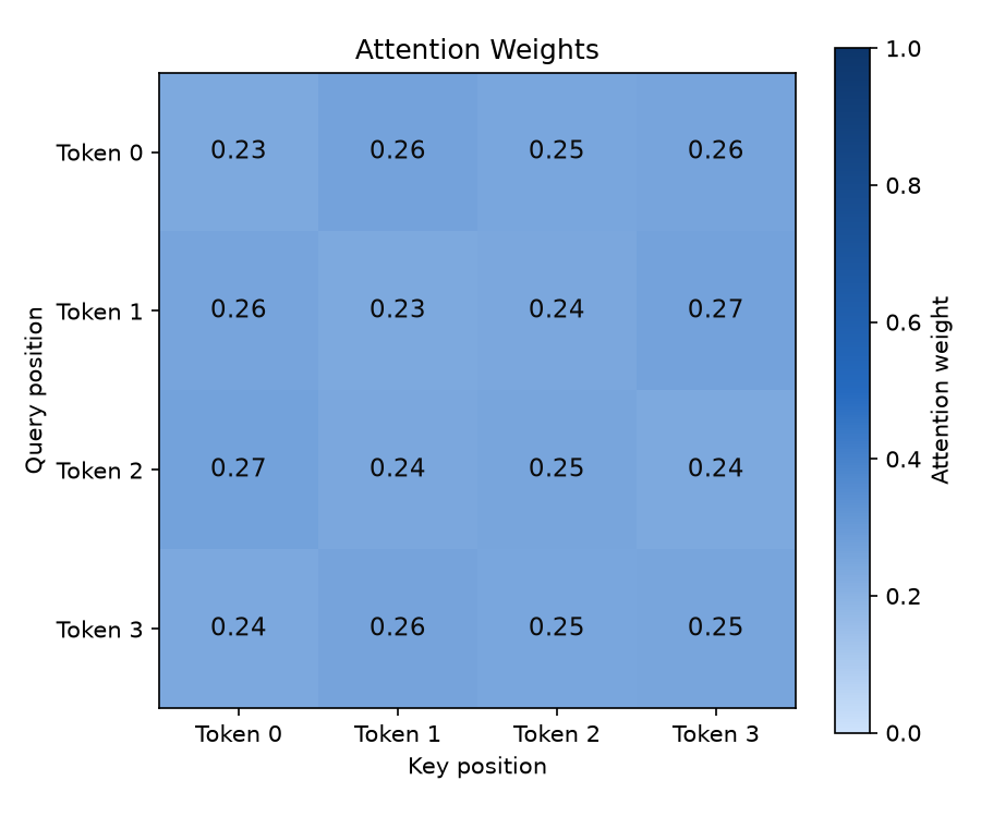
 [[0.235 0.264 0.246 0.255]
  [0.257 0.235 0.244 0.265]
  [0.268 0.243 0.254 0.235]
  [0.242 0.259 0.248 0.251]]
Each row sums to 1.0, as expected from softmax. The weights all fall within the narrow range 0.235-0.268, reflecting the fact that we initialized W_Q and W_K with a small scale of 0.1: the resulting \(QK^T/\sqrt{d_k}\)
values are small, so softmax produces an almost-uniform distribution (after training, the weights would sharpen toward specific tokens). Visualizing it as a heatmap gives:
Multi-Head Attention
Motivation and Formulation
A single attention head can only compute similarities in one representation space. Multi-Head Attention projects Q, K, and V into \(h\) different subspaces and computes attention independently in each, capturing diverse relationships simultaneously.
\[\text{MultiHead}(Q, K, V) = \text{Concat}(\text{head}_1, \ldots, \text{head}_h)W_O \tag{7}\] \[\text{head}_i = \text{Attention}(QW_Q^i, KW_K^i, VW_V^i) \tag{8}\]The standard choice is \(d_k = d_v = d_{\text{model}} / h\) for each head. \(W_O \in \mathbb{R}^{hd_v \times d_{\text{model}}}\) is the output projection matrix. The total parameter count remains roughly the same as single-head attention, but the model can attend to different aspects of the input in different subspaces.
NumPy Implementation
class MultiHeadAttention:
    """Multi-Head Attention (Eqs. 7, 8)"""

    def __init__(self, d_model, n_heads, seed=0):
        assert d_model % n_heads == 0
        self.d_model = d_model
        self.n_heads = n_heads
        self.d_k = d_model // n_heads

        rng = np.random.RandomState(seed)
        scale = 0.1

        # Projection matrices for each head
        self.W_Q = rng.randn(n_heads, d_model, self.d_k) * scale
        self.W_K = rng.randn(n_heads, d_model, self.d_k) * scale
        self.W_V = rng.randn(n_heads, d_model, self.d_k) * scale
        # Output projection matrix
        self.W_O = rng.randn(n_heads * self.d_k, d_model) * scale

    def forward(self, X):
        """
        Parameters:
            X: Input sequence (n, d_model)
        Returns:
            output: Multi-Head Attention output (n, d_model)
            all_weights: Attention weights per head (n_heads, n, n)
        """
        head_outputs = []
        all_weights = []

        for i in range(self.n_heads):
            Q = X @ self.W_Q[i]
            K = X @ self.W_K[i]
            V = X @ self.W_V[i]
            head_out, weights = scaled_dot_product_attention(Q, K, V)
            head_outputs.append(head_out)
            all_weights.append(weights)

        # Concatenate heads and apply output projection (Eq. 7)
        concat = np.concatenate(head_outputs, axis=-1)
        output = concat @ self.W_O

        return output, np.array(all_weights)
Visualizing Multi-Head Attention
np.random.seed(42)

n_tokens = 6
d_model = 16
n_heads = 4

X = np.random.randn(n_tokens, d_model)
mha = MultiHeadAttention(d_model, n_heads, seed=42)
output, all_weights = mha.forward(X)

print("Input shape:", X.shape)
print("Output shape:", output.shape)
print("Attention weights shape:", all_weights.shape)

# Visualize attention weights for each head
fig, axes = plt.subplots(1, n_heads, figsize=(16, 4))
for h in range(n_heads):
    im = axes[h].imshow(all_weights[h], cmap="Blues", vmin=0, vmax=1)
    axes[h].set_title(f"Head {h}")
    axes[h].set_xlabel("Key")
    axes[h].set_ylabel("Query")

plt.suptitle("Multi-Head Attention Weights", fontsize=14)
plt.tight_layout()
plt.show()
Output:
Input shape: (6, 16)
Output shape: (6, 16)
Attention weights shape: (4, 6, 6)
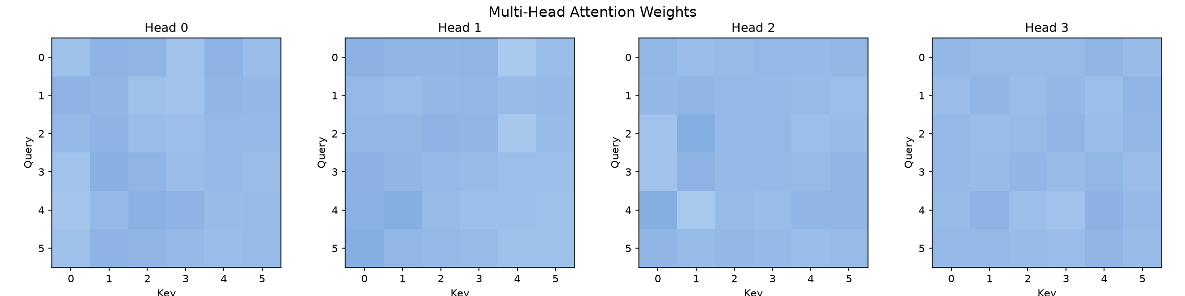
Head 0: mean diagonal=0.1578, max weight=0.2063
Head 1: mean diagonal=0.1646, max weight=0.2142
Head 2: mean diagonal=0.1732, max weight=0.2187
Head 3: mean diagonal=0.1729, max weight=0.1976
The position of the maximum weight (which token each head attends to most) differs across the four heads, confirming that each head learns different relationships in its own independent subspace. Visualizing the four heads side by side makes the difference in shading patterns visually apparent as well.
Positional Encoding
Self-Attention is permutation-invariant: changing the order of tokens yields the same set of outputs. To inject positional information into the sequence, we need Positional Encoding.
The original Transformer paper proposes sinusoidal positional encoding:
\[PE_{(pos, 2i)} = \sin\left(\frac{pos}{10000^{2i/d_{\text{model}}}}\right) \tag{9}\] \[PE_{(pos, 2i+1)} = \cos\left(\frac{pos}{10000^{2i/d_{\text{model}}}}\right) \tag{10}\]Here, \(pos\) is the position in the sequence and \(i\) is the dimension index. Each dimension uses a sinusoidal wave with a different frequency, generating a unique pattern for each position.
Implementation and Visualization
def positional_encoding(max_len, d_model):
    """
    Sinusoidal Positional Encoding (Eqs. 9, 10)

    Parameters:
        max_len: Maximum sequence length
        d_model: Model dimension
    Returns:
        PE: Positional encoding matrix (max_len, d_model)
    """
    PE = np.zeros((max_len, d_model))
    position = np.arange(max_len)[:, np.newaxis]
    div_term = 10000 ** (2 * np.arange(d_model // 2) / d_model)

    PE[:, 0::2] = np.sin(position / div_term)
    PE[:, 1::2] = np.cos(position / div_term)
    return PE

# Visualize positional encoding
max_len = 50
d_model = 64
PE = positional_encoding(max_len, d_model)

fig, ax = plt.subplots(figsize=(10, 6))
im = ax.imshow(PE, cmap="RdBu", aspect="auto")
ax.set_xlabel("Dimension")
ax.set_ylabel("Position")
ax.set_title("Sinusoidal Positional Encoding")
plt.colorbar(im, ax=ax)
plt.tight_layout()
plt.show()
Output:
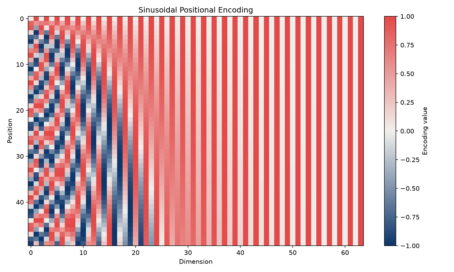
PE shape: (50, 64)
PE range: -0.9999902065507035 1.0
The range is correctly bounded to \([-1, 1]\) (the range of \(\sin\) and \(\cos\) themselves). Visualizing it shows narrower stripes (shorter periods) in the low-dimension columns on the left and near-uniform coloring (longer periods) in the high-dimension columns on the right. This happens because the denominator \(10000^{2i/d_{\text{model}}}\) grows exponentially with \(i\) , so the angular frequency \(1/10000^{2i/d_{\text{model}}}\) shrinks accordingly. Low dimensions carry high frequencies (distinguishing nearby positions) while high dimensions carry low frequencies (encoding coarse, global position), together encoding positional information at multiple scales simultaneously.
Comparison with PyTorch nn.MultiheadAttention
PyTorch provides a built-in nn.MultiheadAttention. Here we set identical weights in both our scratch implementation and PyTorch’s module, and verify that the outputs match.
import torch
import torch.nn as nn

np.random.seed(42)
torch.manual_seed(42)

n_tokens = 4
d_model = 8
n_heads = 2
d_k = d_model // n_heads

# Input data
X_np = np.random.randn(n_tokens, d_model).astype(np.float32)

# --- Scratch implementation ---
mha_np = MultiHeadAttention(d_model, n_heads, seed=0)
out_np, _ = mha_np.forward(X_np)

# --- PyTorch implementation ---
mha_pt = nn.MultiheadAttention(d_model, n_heads, bias=False, batch_first=False)

# Copy weights from scratch implementation into PyTorch's in_proj_weight
# PyTorch stores [W_Q; W_K; W_V] concatenated as (3*d_model, d_model)
W_Q_cat = np.concatenate([mha_np.W_Q[i] for i in range(n_heads)], axis=1).T
W_K_cat = np.concatenate([mha_np.W_K[i] for i in range(n_heads)], axis=1).T
W_V_cat = np.concatenate([mha_np.W_V[i] for i in range(n_heads)], axis=1).T
in_proj_weight = np.concatenate([W_Q_cat, W_K_cat, W_V_cat], axis=0)

with torch.no_grad():
    mha_pt.in_proj_weight.copy_(torch.from_numpy(in_proj_weight))
    mha_pt.out_proj.weight.copy_(torch.from_numpy(mha_np.W_O.T))

# PyTorch expects (seq_len, batch, d_model) by default
X_pt = torch.from_numpy(X_np).unsqueeze(1)  # (n_tokens, 1, d_model)
out_pt, _ = mha_pt(X_pt, X_pt, X_pt)
out_pt = out_pt.squeeze(1).detach().numpy()

# Compare outputs
print("Scratch output:\n", np.round(out_np, 4))
print("PyTorch output:\n", np.round(out_pt, 4))
print("Max difference:", np.max(np.abs(out_np - out_pt)))
print("Mean absolute difference:", np.mean(np.abs(out_np - out_pt)))
Output (run with PyTorch 2.13.0):
Scratch output:
 [[ 0.0045 -0.0228 -0.0071 -0.002   0.0275  0.0026  0.0413  0.0183]
  [-0.0006 -0.0256 -0.0029 -0.0008  0.0284  0.0037  0.037   0.0159]
  [-0.0015 -0.0284  0.0014  0.0004  0.0314  0.0022  0.04    0.0165]
  [ 0.001  -0.0254 -0.0037 -0.0016  0.0283 -0.0009  0.0425  0.0201]]
PyTorch output:
 [[ 0.0045 -0.0228 -0.0071 -0.002   0.0275  0.0026  0.0413  0.0183]
  [-0.0006 -0.0256 -0.0029 -0.0008  0.0284  0.0037  0.037   0.0159]
  [-0.0015 -0.0284  0.0014  0.0004  0.0314  0.0022  0.04    0.0165]
  [ 0.001  -0.0254 -0.0037 -0.0016  0.0283 -0.0009  0.0425  0.0201]]
Max difference: 5.749276447281071e-09
Mean absolute difference: 2.097602618178127e-09
At 4 decimal places the two outputs are identical, and even before rounding the maximum absolute difference is \(5.7 \times 10^{-9}\)
with a mean absolute difference of \(2.1 \times 10^{-9}\)
— well within float32 rounding error (typically \(10^{-7}\)
to \(10^{-8}\)
). This is empirical confirmation that the NumPy scratch implementation and PyTorch’s internal implementation (which routes through the optimized F.scaled_dot_product_attention matrix operations) compute mathematically identical functions.
Intuitive Understanding of Attention
The essence of Self-Attention is a data-dependent weighted average.
In conventional filters (such as moving averages or EMA ), the weights are predetermined and independent of the input. In Self-Attention, however, the weights (the attention matrix \(A\) ) are computed from the input \(X\) itself.
| Property | Fixed-weight filters | Self-Attention |
|---|---|---|
| Weight assignment | Fixed in advance | Dynamically computed from input |
| Reference range | Local (window-dependent) | Global (entire sequence) |
| Adaptivity | None | Weights change per input |
| Complexity | \(O(n)\) | \(O(n^2)\) (quadratic in sequence length) |
| Use cases | Signal smoothing, denoising | Sequence relationship modeling |
This “input-dependent dynamic weighting” is the source of Attention’s power. Each token can selectively decide which other tokens to attend to based on context, enabling the model to capture long-range dependencies and complex structures flexibly.
Efficient Attention: Recent Research Trends
As the table above shows, Self-Attention’s computational cost scales as \(O(n^2)\) in the sequence length \(n\) . Computing \(S = QK^T\) from Eq. (3) naively requires holding the entire \(n \times n\) matrix in memory, so as \(n\) grows (long documents, genomic sequences, and so on), both memory and runtime become bottlenecks. Since 2023, several practical solutions to this problem have become established.
FlashAttention (Dao et al., 2022; NeurIPS 2022) is an IO-aware algorithm that, without changing the mathematical result of Attention at all (it is exact, not an approximation), tiles the computation to exploit the GPU memory hierarchy — fast, small-capacity SRAM versus slow, large-capacity HBM — and computes the result with an online softmax (updating running partial sums and maxima block by block) so the full \(n \times n\) matrix \(S\) is never materialized in HBM. Its successor, FlashAttention-2 (Dao, 2023; arXiv:2307.08691), improves GPU work partitioning and parallelism to reach 50-73% of theoretical peak FLOPs/s on an A100, and FlashAttention-3 (Shah et al., 2024; arXiv:2407.08608) exploits asynchronous execution and FP8 low-precision computation on H100 GPUs for a further 1.5-2.0x speedup. Equation (2) itself is unchanged — the gains come purely from implementation-level engineering of how the computation is carried out, yet they are substantial in both speed and memory footprint.
A second, complementary direction changes how Multi-Head Attention (Eqs. 7, 8) holds its Key and Value tensors:
- Multi-Query Attention (MQA) (Shazeer, 2019): all heads share a single Key and Value, with only the Query kept per-head. This shrinks the inference-time KV cache by a factor of \(h\) , but was reported to cause quality degradation from the reduced representational capacity.
- Grouped-Query Attention (GQA) (Ainslie et al., 2023; arXiv:2305.13245): an intermediate design between MHA and MQA. The \(h\) Query heads are split into \(g\) groups, and heads within a group share Key/Value projections (\(g=1\) recovers MQA; \(g=h\) recovers standard MHA). The paper shows that an existing MHA checkpoint can be converted to GQA with a small amount of additional fine-tuning, compressing the KV cache by a factor of \(h/g\) with minimal quality loss — which is why GQA has been adopted in many large language models, including LLaMA 2 and Mistral 7B.
The scratch implementation in this article (the MultiHeadAttention class) is a standard MHA where every head keeps its own independent W_K and W_V. Extending it to GQA requires only grouping the heads and sharing W_K[i]/W_V[i] within each group — the structure of Eq. (8) itself carries over unchanged. Note that the practical compute-cost tradeoffs of applying Transformers to long time-series sequences are touched on briefly in
Transformers for Time Series Forecasting
; this article instead focuses on the algorithmic mechanics of FlashAttention, GQA, and MQA themselves.
Summary
- Self-Attention dynamically computes the relevance between all pairs of elements in a sequence to produce context-aware representations
- Scaled Dot-Product Attention computes Query-Key dot products, scales by \(\sqrt{d_k}\) , applies softmax to obtain attention weights, and computes a weighted sum of Values
- Multi-Head Attention computes attention independently in multiple subspaces, capturing diverse patterns simultaneously
- Positional Encoding injects position information into the permutation-invariant Self-Attention mechanism
- The essence of Attention is a data-dependent weighted average, fundamentally different from fixed-weight filters
- FlashAttention computes the exact same result faster and with less memory via IO-aware tiling, while GQA/MQA shrink the KV cache by sharing Key/Value projections across heads
Related Articles
- From SGD to Adam: Evolution of Gradient-Based Optimization - Covers the optimization methods used to train Transformers.
- Ensemble Learning: From Decision Trees to Random Forest and Gradient Boosting - Covers ensemble methods as an alternative machine learning approach.
- Support Vector Machines (SVM): Kernel Methods and Nonlinear Classification with Python - Deepens understanding of the similarity between kernel tricks and Attention.
- k-means and GMM: Clustering Theory and Python Implementation - Representative unsupervised learning methods.
- Frequency Characteristics of the EMA Filter - A reference for understanding the contrast between fixed-weight filters and dynamic attention weights.
- Moving Average Filters Compared: SMA, WMA, and EMA in Python - A reference for contrasting Attention with fixed-weight filters.
- Transformers for Time Series Forecasting - Covers practical compute-cost considerations when applying Transformers to long sequences.
References
- Vaswani, A., et al. (2017). “Attention Is All You Need.” NeurIPS 2017.
- PyTorch Documentation:
nn.MultiheadAttention. https://pytorch.org/docs/stable/generated/torch.nn.MultiheadAttention.html - Alammar, J. (2018). “The Illustrated Transformer.” https://jalammar.github.io/illustrated-transformer/
- Dao, T., Fu, D. Y., Ermon, S., Rudra, A., & Ré, C. (2022). “FlashAttention: Fast and Memory-Efficient Exact Attention with IO-Awareness.” NeurIPS 2022. https://arxiv.org/abs/2205.14135
- Dao, T. (2023). “FlashAttention-2: Faster Attention with Better Parallelism and Work Partitioning.” arXiv:2307.08691. https://arxiv.org/abs/2307.08691
- Shah, J., et al. (2024). “FlashAttention-3: Fast and Accurate Attention with Asynchrony and Low-precision.” arXiv:2407.08608. https://arxiv.org/abs/2407.08608
- Shazeer, N. (2019). “Fast Transformer Decoding: One Write-Head is All You Need.” arXiv:1911.02150. https://arxiv.org/abs/1911.02150
- Ainslie, J., Lee-Thorp, J., de Jong, M., Zemlyanskiy, Y., Lebrón, F., & Sanghai, S. (2023). “GQA: Training Generalized Multi-Query Transformer Models from Multi-Head Checkpoints.” arXiv:2305.13245. https://arxiv.org/abs/2305.13245