What is CalcBox?
CalcBox is a collection of 61+ free calculators for everyday life. No installation, no sign-up required. Beyond linking to each tool, this article dives into the math behind two of the money calculators — loan repayment and compound interest — deriving their formulas, exposing the numerical pitfalls that arise at a zero interest rate, on leap years, and from floating-point rounding, and verifying everything with Python.
Categories
Life
Split bill, sales tax, electricity cost, unit converter, discount calculator, currency converter, and more.
Health
BMI, calorie burn, body fat percentage, BMR, sleep cycle, alcohol metabolism time, and more.
Money
Loan repayment, compound interest, salary calculator, pension simulator, and more. The next section derives the formulas behind the loan and compound interest calculators in detail.
Date & Time
Days between dates, age calculator, Japanese/Western year converter, timezone converter, countdown timer, and stopwatch.
Developer
Base converter, JSON formatter, regex tester, password generator, hash generator, and more.
Deriving the Loan Amortization and Compound Interest Formulas
We derive the formulas used internally by the loan and compound-interest calculators from the present-value-of-annuity relationship.
The amortization payment from the present value of an annuity
Consider a loan of principal \(P\) , periodic rate \(r\) (e.g. a monthly rate), and \(n\) equal payments \(M\) (level-payment amortization). The present value of the \(k\) -th payment \(M\) is \(M/(1+r)^k\) , so requiring the sum of the present values of all \(n\) payments to equal the principal \(P\) gives
\[ P = \sum_{k=1}^{n} \frac{M}{(1+r)^k} \tag{1} \]The right-hand side is exactly the geometric sum \(\sum_{k=1}^n x^k = x\dfrac{1-x^n}{1-x}\) with \(x = 1/(1+r)\) . Substituting,
\[ \sum_{k=1}^{n} \frac{1}{(1+r)^k} = \frac{1}{1+r} \cdot \frac{1-(1+r)^{-n}}{1-\frac{1}{1+r}} = \frac{1}{1+r} \cdot \frac{1-(1+r)^{-n}}{\frac{r}{1+r}} = \frac{1-(1+r)^{-n}}{r} \tag{2} \]so equation (1) becomes
\[ P = M \cdot \frac{1-(1+r)^{-n}}{r} \tag{3} \]Solving for \(M\) :
\[ M = P \cdot \frac{r}{1-(1+r)^{-n}} = P\, \frac{r(1+r)^n}{(1+r)^n - 1} \tag{4} \]This is the standard level-payment amortization formula used by CalcBox’s loan calculator . Equation (3) is nothing more than the accounting identity “the present value of the level payments equals the principal at origination”; equation (4) simply solves that identity for \(M\) .
Compound interest and the continuous-compounding limit
Investing principal \(P\) at annual rate \(r\) , compounded \(m\) times per year for \(t\) years, gives
\[ A(m) = P\left(1+\frac{r}{m}\right)^{mt} \tag{5} \]As the compounding frequency \(m\) used by the compound interest calculator increases, this converges to the continuous-compounding limit. Setting \(x = r/m\) , \(m \to \infty\) corresponds to \(x \to 0\) , and
\[ A(m) = P\left[(1+x)^{1/x}\right]^{rt} \tag{6} \]Using the defining limit of Euler’s number \(\lim_{x\to 0}(1+x)^{1/x} = e\) ,
\[ \lim_{m\to\infty} A(m) = P \, e^{rt} \tag{7} \]which is the familiar continuous-compounding formula \(A = Pe^{rt}\) . The execution results below show equation (5) converging monotonically to equation (7) as \(m\) is increased from 1 (annual compounding) to one million.
Edge Cases: Where the Formulas Break
Despite their simple appearance, equations (4) and (5) have real numerical pitfalls under specific inputs. We examine three of them.
The zero-rate singularity (a 0/0 indeterminate form)
Substituting \(r=0\)
into equation (4), \(M = P\,r(1+r)^n / ((1+r)^n-1)\)
, gives a numerator of \(0 \cdot 1^n = 0\)
and a denominator of \(1^n - 1 = 0\)
— a 0/0 indeterminate form. Evaluating this formula literally in Python raises a ZeroDivisionError, as confirmed in the execution results below.
The correct limit follows from L’Hôpital’s rule. With numerator \(f(r) = r(1+r)^n\) and denominator \(g(r) = (1+r)^n - 1\) ,
\[ f'(r) = (1+r)^n + n r (1+r)^{n-1}, \qquad g'(r) = n(1+r)^{n-1} \tag{8} \]At \(r=0\) : \(f'(0) = 1\) , \(g'(0) = n\) , so
\[ \lim_{r \to 0} \frac{f(r)}{g(r)} = \frac{f'(0)}{g'(0)} = \frac{1}{n} \tag{9} \]Hence the correct payment as \(r \to 0\) is
\[ M \Big|_{r=0} = \frac{P}{n} \tag{10} \]i.e. the principal divided evenly by the number of payments — which matches the intuition that a zero rate means no interest accrues, so the loan is simply repaid in equal installments. A first-order Taylor expansion \((1+r)^n \approx 1 + nr + \binom{n}{2}r^2\) of both numerator and denominator reaches the same conclusion \(M \to P/n\) , which we verify numerically below.
More importantly for implementations: even before \(r\) reaches exactly zero, for extremely small \(r\) (around \(10^{-12}\) ) the denominator \((1+r)^n - 1\) in equation (4) suffers catastrophic cancellation. Because \((1+r)^n\) is represented in floating point as a value extremely close to 1, subtracting 1 destroys most of the significant digits. The execution results show the formula’s value converging toward \(P/n\) as \(r\) shrinks, then — below roughly \(r < 10^{-10}\) — the error actually growing again due to this cancellation. A robust implementation should branch to equation (10) directly whenever \(r\) falls below a threshold (e.g. \(10^{-8}\) ), rather than relying on equation (4).
Leap years and day-count conventions (30/360 vs. Actual/365 vs. Actual/Actual)
Day-based interest accrual can produce different results for the same nominal rate and same date range, depending on the day-count convention used. The three common conventions are:
| Convention | Numerator (elapsed days) | Denominator (days per year) |
|---|---|---|
| 30/360 | Every month counted as exactly 30 days | Fixed 360 |
| Actual/365 | Actual calendar days | Fixed 365 |
| Actual/Actual | Actual calendar days | Actual days in the year (366 in a leap year) |
Since accrued interest is \(I = P \cdot r \cdot (\text{elapsed days}/\text{denominator days})\) , a period spanning February in a leap year automatically adds one extra day to the Actual-day numerator. The execution results below show that for the leap year 2028’s Jan 15–Mar 15 window (60 actual days, also 60 under 30/360), the three conventions produce interest amounts ranging from ¥81,967 to ¥83,333 — a difference of roughly ¥1,366. For the non-leap year 2027, the same date range has only 59 actual days, and — as verified below — Actual/365 and Actual/Actual then agree exactly.
Accumulated floating-point error: iterative loop vs. closed form
When simulating compound interest, computing “multiply in the daily interest one day at a time in a loop” versus “evaluate the closed-form formula (5) once” can accumulate rounding error differently. At float64 (double precision) the difference is normally negligible, but running the same loop in float32 (single precision) accumulates rounding error over 10,950 multiplications (30 years of daily compounding) into a difference that is far from negligible, as the execution results demonstrate.
Python Implementation and Verification
A 30-year mortgage example
We compute a level-payment amortization for a ¥30,000,000 principal at a 3% annual rate (converted to a monthly rate) over 30 years (360 payments), and verify the full payment schedule.
def amortization_payment(P, r, n):
    """Standard loan amortization formula: M = P r(1+r)^n / ((1+r)^n - 1)"""
    return P * r * (1 + r) ** n / ((1 + r) ** n - 1)


P = 30_000_000.0        # principal, yen
annual_rate = 0.03      # nominal annual rate
n_years = 30
n = n_years * 12         # number of monthly payments
r = annual_rate / 12     # monthly rate

M = amortization_payment(P, r, n)
total_paid = M * n
total_interest = total_paid - P

print(f"P = {P:,.0f} yen, annual rate = {annual_rate:.1%}, n = {n} payments, r = {r:.6f}")
print(f"Monthly payment M = {M:,.2f} yen")
print(f"Total paid = {total_paid:,.2f} yen")
print(f"Total interest = {total_interest:,.2f} yen")

# Build the full schedule to verify the principal/interest split and that the balance hits zero
balance = P
principal_parts, interest_parts, balances = [], [], [P]
for k in range(1, n + 1):
    interest_k = balance * r
    principal_k = M - interest_k
    balance -= principal_k
    principal_parts.append(principal_k)
    interest_parts.append(interest_k)
    balances.append(balance)

print(f"Final balance after {n} payments: {balance:.10f} yen (should be ~0)")
print(f"Sum of principal parts: {sum(principal_parts):,.2f} yen (should equal P = {P:,.2f})")
print(f"Sum of interest parts:  {sum(interest_parts):,.2f} yen (should equal total_interest = {total_interest:,.2f})")
print(f"First payment: principal={principal_parts[0]:.2f}, interest={interest_parts[0]:.2f}")
print(f"Last payment (n={n}): principal={principal_parts[-1]:.2f}, interest={interest_parts[-1]:.2f}")
Execution result:
P = 30,000,000 yen, annual rate = 3.0%, n = 360 payments, r = 0.002500
Monthly payment M = 126,481.21 yen
Total paid = 45,533,235.64 yen
Total interest = 15,533,235.64 yen
Final balance after 360 payments: -0.0000009574 yen (should be ~0)
Sum of principal parts: 30,000,000.00 yen (should equal P = 30,000,000.00)
Sum of interest parts:  15,533,235.64 yen (should equal total_interest = 15,533,235.64)
First payment: principal=51481.21, interest=75000.00
Last payment (n=360): principal=126165.80, interest=315.41
The final balance, which should theoretically be exactly zero, comes out to \(-9.57 \times 10^{-7}\) yen — a tiny floating-point artifact from accumulated rounding over 360 subtractions, negligible in practice. The principal and interest totals match the total principal and total interest exactly, confirming equation (4)’s derivation empirically. The first payment’s interest (¥75,000) exceeds its principal (¥51,481), while the last payment’s principal (¥126,166) dominates with only ¥315 of interest remaining — confirming the well-known property that level-payment loans are interest-heavy early and principal-heavy late.
Verifying the zero-rate limit
We check what happens evaluating equation (4) literally at \(r=0\) , compare it against the correct limit from equation (10), and trace the convergence as \(r \to 0\) .
# Plugging r=0 directly into equation (4)
r_zero = 0.0
numerator = r_zero * (1 + r_zero) ** n
denominator = (1 + r_zero) ** n - 1
print(f"r=0: numerator={numerator}, denominator={denominator}")

try:
    bad = numerator / denominator
except ZeroDivisionError as e:
    print(f"ZeroDivisionError raised: {e}")

# Correct limit
limit_formula = P / n
print(f"Correct limit (L'Hopital): M = P/n = {limit_formula:.6f}")

# Convergence as r -> 0
for rr in [1e-2, 1e-4, 1e-6, 1e-8, 1e-10, 1e-12]:
    val = amortization_payment(P, rr, n)
    print(f"  r={rr:<10g}  M(r)={val:.8f}  diff from P/n = {val - limit_formula:.3e}")

for rr in [1e-14, 1e-16, 0.0]:
    denom = (1 + rr) ** n - 1
    if denom == 0:
        print(f"  r={rr:<10g}  (1+r)^n - 1 = 0.0 in floating point -> equation (4) divides by zero")
    else:
        val = amortization_payment(P, rr, n)
        print(f"  r={rr:<10g}  M(r)={val:.8f}  denom={denom:.3e}")
Execution result:
r=0: numerator=0.0, denominator=0.0
ZeroDivisionError raised: division by zero
Correct limit (L'Hopital): M = P/n = 83333.333333
  r=0.01        M(r)=308583.77907765  diff from P/n = 2.253e+05
  r=0.0001      M(r)=84846.49928623  diff from P/n = 1.513e+03
  r=1e-06       M(r)=83348.37590683  diff from P/n = 1.504e+01
  r=1e-08       M(r)=83333.48425806  diff from P/n = 1.509e-01
  r=1e-10       M(r)=83333.32789633  diff from P/n = -5.437e-03
  r=1e-12       M(r)=83325.92564002  diff from P/n = -7.408e+00
  r=1e-14       M(r)=83399.99309975  denom=3.597e-12
  r=1e-16       (1+r)^n - 1 = 0.0 in floating point -> equation (4) divides by zero
  r=0           (1+r)^n - 1 = 0.0 in floating point -> equation (4) divides by zero
As expected, the literal \(r=0\)
evaluation raises ZeroDivisionError. Shrinking \(r\)
from \(10^{-2}\)
down to \(10^{-10}\)
, equation (4)’s value converges monotonically toward \(P/n = 83{,}333.33\)
yen (the difference shrinks by roughly an order of magnitude each step: \(2.25\times10^5 \to 1.51\times10^3 \to 1.50\times10^1 \to 1.51\times10^{-1} \to -5.44\times10^{-3}\)
). But at \(r=10^{-12}\)
the difference grows back out to \(-7.41\)
, and at \(r=10^{-14}\)
–\(10^{-16}\)
and at \(r=0\)
, the denominator \((1+r)^n - 1\)
collapses to exactly zero in floating point. This is the catastrophic-cancellation effect described above in action: a quantity that mathematically converges as \(r\to 0\)
actually gets worse numerically past a certain point. In production code, the safe approach is to branch to \(P/n\)
directly whenever \(r\)
falls below a threshold such as \(10^{-8}\)
, rather than trusting equation (4) all the way down to zero.
Comparing day-count conventions
For the leap year 2028 and the non-leap year 2027, we apply the same Jan 15–Mar 15 date range and 5% annual rate under all three day-count conventions and compare the resulting interest.
import datetime


def days_30_360(d1, d2):
    """Simplified US (NASD) 30/360 convention."""
    d1_day = min(d1.day, 30)
    d2_day = min(d2.day, 30) if d1_day == 30 else d2.day
    return (d2.year - d1.year) * 360 + (d2.month - d1.month) * 30 + (d2_day - d1_day)


def is_leap(y):
    return (y % 4 == 0 and y % 100 != 0) or (y % 400 == 0)


principal_dc = 10_000_000.0
annual_rate_dc = 0.05

for d1, d2 in [
    (datetime.date(2028, 1, 15), datetime.date(2028, 3, 15)),  # leap year
    (datetime.date(2027, 1, 15), datetime.date(2027, 3, 15)),  # non-leap year
]:
    days_360 = days_30_360(d1, d2)
    days_act = (d2 - d1).days
    year_days = 366 if is_leap(d1.year) else 365

    interest_30_360 = principal_dc * annual_rate_dc * days_360 / 360
    interest_act_365 = principal_dc * annual_rate_dc * days_act / 365
    interest_act_actual = principal_dc * annual_rate_dc * days_act / year_days

    print(f"Period: {d1} to {d2} ({d1.year} is a leap year: {is_leap(d1.year)})")
    print(f"  30/360 day count: {days_360} days,  actual days: {days_act} days")
    print(f"  Interest (30/360)       : {interest_30_360:,.4f} yen")
    print(f"  Interest (Actual/365)   : {interest_act_365:,.4f} yen")
    print(f"  Interest (Actual/Actual): {interest_act_actual:,.4f} yen")
Execution result:
Period: 2028-01-15 to 2028-03-15 (2028 is a leap year: True)
  30/360 day count: 60 days,  actual days: 60 days
  Interest (30/360)       : 83,333.3333 yen
  Interest (Actual/365)   : 82,191.7808 yen
  Interest (Actual/Actual): 81,967.2131 yen
Period: 2027-01-15 to 2027-03-15 (2027 is a leap year: False)
  30/360 day count: 60 days,  actual days: 59 days
  Interest (30/360)       : 83,333.3333 yen
  Interest (Actual/365)   : 80,821.9178 yen
  Interest (Actual/Actual): 80,821.9178 yen
Despite the same ¥10,000,000 principal, 5% annual rate, and identical Jan 15–Mar 15 date range, the interest ranges from ¥81,967 to ¥83,333 depending on convention — a difference of about ¥1,366 (\(83{,}333.33 - 81{,}967.21\) ). Interestingly, in leap year 2028 the day count itself doesn’t differ between 30/360 and Actual (both 60 days) — the difference comes purely from the denominator (360 vs. 365 vs. 366 fixed days). In non-leap 2027, actual days drop to 59, and since both Actual/365 and Actual/Actual then use the same 365-day denominator, their interest amounts match exactly (¥80,821.9178). Because lenders differ in which convention they use, the same quoted “5% annual rate” can produce measurably different actual interest.
Comparing precision: iterative loop vs. closed form
We compare a “multiply in one day of interest at a time, in a loop” implementation of daily compounding against a single closed-form evaluation, at both float64 and float32 precision.
import numpy as np

P_fp = 1_000_000.0
daily_rate = 0.05 / 365
n_days = 365 * 30  # 30 years of daily compounding

# Closed form, float64
closed_form_64 = P_fp * (1 + daily_rate) ** n_days

# Iterative loop, float64
balance64 = np.float64(P_fp)
for _ in range(n_days):
    balance64 = balance64 * (np.float64(1.0) + np.float64(daily_rate))

# Iterative loop, float32 (single precision)
balance32 = np.float32(P_fp)
rate32 = np.float32(daily_rate)
for _ in range(n_days):
    balance32 = balance32 * (np.float32(1.0) + rate32)

print(f"n_days = {n_days}")
print(f"Closed-form (float64):        {closed_form_64:.6f}")
print(f"Iterative loop (float64):     {balance64:.6f}")
print(f"Iterative loop (float32):     {float(balance32):.6f}")
print(f"Diff closed-form vs iter64:    {closed_form_64 - balance64:.10f}")
print(f"Diff closed-form vs iter32:    {closed_form_64 - float(balance32):.6f}")
print(f"Relative diff (float32 case): {(closed_form_64 - float(balance32)) / closed_form_64:.3e}")
Execution result:
n_days = 10950
Closed-form (float64):        4481228.688523
Iterative loop (float64):     4481228.688523
Iterative loop (float32):     4480501.000000
Diff closed-form vs iter64:    0.0000000289
Diff closed-form vs iter32:    727.688523
Relative diff (float32 case): 1.624e-04
Comparing float64 closed-form to float64 iterative loop, the difference is a mere \(2.89 \times 10^{-8}\) yen — practically zero. But running the exact same algorithm in float32 (single precision) accumulates rounding error over 10,950 multiplications into a difference of ¥727.69 from the closed form, a relative error of \(1.6\times10^{-4}\) . A ¥727 drift on a ¥1,000,000 principal is not negligible at household-budget scale, and shows the real risk: if float32 gets used unintentionally (e.g. via GPU tensors or a NumPy default dtype) for a long-running daily-compounding simulation, the error accumulates silently. The safe practice for financial calculations is to evaluate the closed-form expression directly whenever possible, or, if iteration is required, to explicitly use float64 or higher precision.
Convergence to continuous compounding
We also verify that equation (5) converges to the continuous-compounding formula (7) as the compounding frequency \(m\) increases.
P_ci = 1_000_000.0
r_annual = 0.05
t_years = 10

for m in [1, 2, 4, 12, 52, 365, 8760, 1_000_000]:
    A = P_ci * (1 + r_annual / m) ** (m * t_years)
    print(f"  m={m:<10d} A = {A:.6f}")

A_continuous = P_ci * np.exp(r_annual * t_years)
print(f"  continuous (Pe^rt)   A = {A_continuous:.6f}")
  m=1          A = 1628894.626777
  m=2          A = 1638616.440290
  m=4          A = 1643619.463487
  m=12         A = 1647009.497690
  m=52         A = 1648325.244915
  m=365        A = 1648664.813765
  m=8760       A = 1648718.918078
  m=1000000    A = 1648721.248742
  continuous (Pe^rt)   A = 1648721.270700
From ¥1,628,894.63 at annual compounding (\(m=1\) ), the value increases monotonically as compounding frequency increases, reaching ¥1,648,721.25 at \(m=1{,}000{,}000\) (essentially continuous), a difference of just ¥0.02 from the theoretical continuous-compounding value \(Pe^{rt} = \text{¥}1{,}648{,}721.27\) . This confirms numerically that the limit derived in equation (7) is correct.
Figures: amortization schedule and day-count comparison
For the 30-year mortgage example above, we plot the principal/interest breakdown of each payment and the loan balance over time.
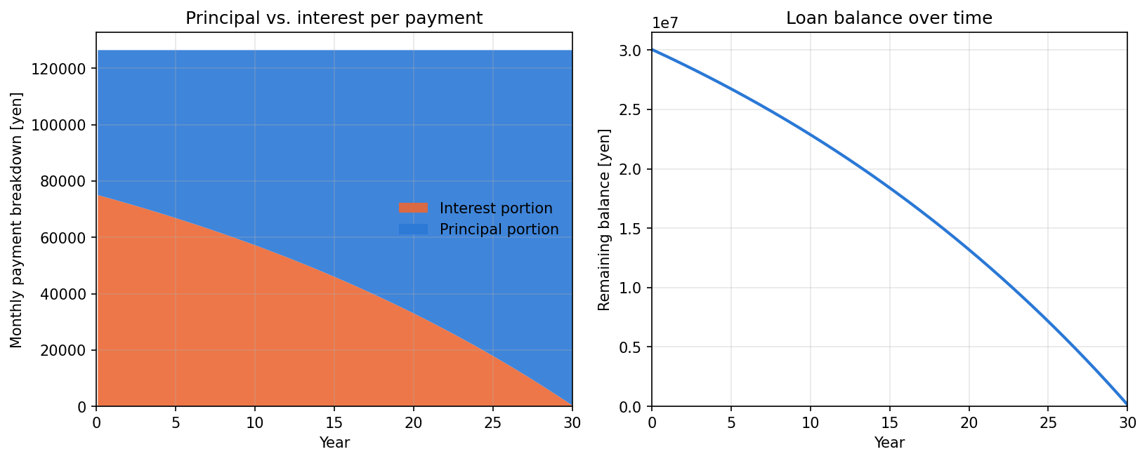
The left panel shows how each year’s (constant) monthly payment splits between principal (blue) and interest (orange) — heavily interest-weighted at the start, shifting to principal-weighted by the end, the classic shape of level-payment amortization. The right panel shows the balance smoothly decaying to zero over the 30-year term.
We also visualize the effect of day-count convention on computed interest.
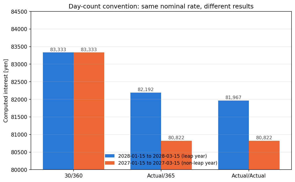
For both the leap year (2028, blue) and the non-leap year (2027, orange), the chart compares interest computed under the three conventions. The 30/360 convention produces the same ¥83,333 in both years, while the Actual-based conventions yield less interest in the leap year (because the denominator becomes 366 days), and Actual/365 and Actual/Actual coincide exactly in the non-leap year.
Key Features
- Free & No Registration
- Mobile-Friendly
- Bilingual - Japanese and English
- PWA Support - Install as an app
Summary
- The level-payment amortization formula \(M = P\,r(1+r)^n/((1+r)^n-1)\) is simply the present-value-of-annuity identity \(P = \sum_{k=1}^n M/(1+r)^k\) solved for \(M\)
- The compound interest formula \(A=P(1+r/m)^{mt}\) reduces to the continuous-compounding formula \(A=Pe^{rt}\) in the limit \(m\to\infty\) , via the defining limit \(\lim_{x\to0}(1+x)^{1/x}=e\)
- At \(r=0\)
the loan amortization formula is a \(0/0\)
indeterminate form, but L’Hôpital’s rule gives the correct limit as the simple \(P/n\)
— confirmed both algebraically and by observing an actual
ZeroDivisionError - For extremely small \(r\) (around \(10^{-12}\) ), a quantity that mathematically converges as \(r\to0\) actually gets numerically worse due to floating-point catastrophic cancellation, as verified experimentally
- Day-count conventions (30/360, Actual/365, Actual/Actual) produce measurably different interest — up to about ¥1,366 in our test — for the same nominal rate and date range
- Simulating daily compounding in float32 accumulates rounding error to a ¥727 (relative error \(1.6\times10^{-4}\) ) difference from the closed form — financial calculations should favor closed-form evaluation, or float64+ precision when iterating
Try CalcBox today.
Related tools: DevToolBox - Developer Tools | Pomodoro Timer
References
- Fabozzi, F. J. (2012). Bond Markets, Analysis, and Strategies (8th ed.). Pearson. (Standard derivation of present-value-of-annuity and level-payment amortization.)
- ISDA (2006). 2006 ISDA Definitions, Section 4.16 (Day Count Fraction). (Industry-standard definitions of 30/360, Actual/365, Actual/Actual, and other day-count conventions.)
- Goldberg, D. (1991). “What Every Computer Scientist Should Know About Floating-Point Arithmetic.” ACM Computing Surveys, 23(1), 5-48. (Classic reference on floating-point cancellation and precision.)