What Are Adaptive Filters?
An adaptive filter automatically adjusts its coefficients to track changes in the statistical properties of input signals. Unlike fixed-parameter filters such as EMA or Butterworth filters , adaptive filters can perform optimally in unknown or dynamically changing environments.
Key Applications
- Noise cancellation: Removing environmental noise captured by microphones (ANC headphones)
- Echo cancellation: Eliminating echoes in phone calls and video conferences
- System identification: Estimating the transfer function of an unknown system
- Channel equalization: Compensating for transmission path distortion in communications
This article focuses on a comparative overview and practical implementation (a verified noise-cancellation experiment) of the three major adaptive filtering algorithms — LMS, NLMS, and RLS. The rigorous theory behind each algorithm — convergence proofs, quantified misadjustment, and the equivalence to the Kalman filter — is left to companion articles ( LMS and NLMS Algorithms: Theory and Python Implementation and The RLS Algorithm in Python ). Toward the end, this article covers practical pitfalls those companion articles don’t address — choosing the filter order, the step-size/steady-error trade-off, and reference-signal correlation issues — each backed by executed code. For the derivation of the Wiener-Hopf equation from steepest descent, see Adaptive Filter Theory and Applications in Digital Signal Processing .
Relationship to the Wiener Filter
The theoretical foundation of adaptive filters is the Wiener filter . The Wiener filter minimizes the mean squared error (MSE) when estimating a desired signal \(d(n)\) from an input signal \(\mathbf{x}(n)\) .
With filter output \(y(n) = \mathbf{w}^T \mathbf{x}(n)\) and error \(e(n) = d(n) - y(n)\) , the MSE is:
\[ J(\mathbf{w}) = E[e^2(n)] = E[(d(n) - \mathbf{w}^T \mathbf{x}(n))^2] \tag{1} \]The optimal solution (Wiener-Hopf solution) is:
\[ \mathbf{w}^* = \mathbf{R}^{-1} \mathbf{p} \tag{2} \]where \(\mathbf{R} = E[\mathbf{x}(n)\mathbf{x}^T(n)]\) is the input autocorrelation matrix and \(\mathbf{p} = E[\mathbf{x}(n)d(n)]\) is the cross-correlation vector. Since \(\mathbf{R}\) and \(\mathbf{p}\) are typically unknown or time-varying, adaptive algorithms iteratively approach the Wiener solution. The derivation of Eq. (2) — expanding \(J(\mathbf{w})\) and setting its derivative with respect to \(\mathbf{w}\) to zero — is covered in detail, alongside steepest descent, in Adaptive Filter Theory and Applications in Digital Signal Processing .
LMS (Least Mean Squares) Algorithm
The LMS algorithm approximates the MSE gradient using instantaneous estimates — a form of stochastic gradient descent, sharing the same principles as SGD .
Derivation
The gradient of \(J(\mathbf{w})\) is:
\[ \nabla J(\mathbf{w}) = -2E[\mathbf{x}(n)e(n)] \tag{3} \]LMS replaces the expectation with instantaneous values:
\[ \hat{\nabla} J(\mathbf{w}) = -2\mathbf{x}(n)e(n) \tag{4} \]The update rule becomes:
\[ \mathbf{w}(n+1) = \mathbf{w}(n) + \mu \mathbf{x}(n) e(n) \tag{5} \]where \(\mu\) is the step size (learning rate).
Convergence Condition
For LMS to converge, the step size must satisfy:
\[ 0 < \mu < \frac{2}{\lambda_{\max}} \tag{6} \]where \(\lambda_{\max}\) is the largest eigenvalue of \(\mathbf{R}\) . In practice:
\[ 0 < \mu < \frac{2}{M \cdot \sigma_x^2} \tag{7} \]where \(M\) is the filter order and \(\sigma_x^2\) is the input signal power. The convergence condition in Eq. (6) can be proven rigorously from the recursion of the weight-error vector, and the residual steady-state error (misadjustment) can be quantified as well — that derivation is left to LMS and NLMS Algorithms: Theory and Python Implementation .
NLMS (Normalized LMS) Algorithm
LMS’s convergence depends on input signal power. NLMS normalizes by the input vector norm:
\[ \mathbf{w}(n+1) = \mathbf{w}(n) + \frac{\mu}{\|\mathbf{x}(n)\|^2 + \epsilon} \mathbf{x}(n) e(n) \tag{8} \]where \(\epsilon\) is a small positive constant to prevent division by zero. With NLMS, convergence is guaranteed for \(0 < \mu < 2\) . Equation (8) looks like it is asserted without justification, but it can actually be derived from the minimum disturbance principle — choosing the update that drives the a posteriori error to exactly zero while moving the weights as little as possible. That derivation, and how the NLMS step size trades off against steady-state error (which this article also verifies numerically further below), is covered in LMS and NLMS Algorithms: Theory and Python Implementation .
RLS (Recursive Least Squares) Algorithm
RLS minimizes the weighted least squares error over all past data. It converges faster than LMS but has higher computational cost.
Cost Function
\[ J(\mathbf{w}, n) = \sum_{i=1}^{n} \lambda^{n-i} |e(i)|^2 \tag{9} \]where \(\lambda\) (\(0 < \lambda \le 1\) ) is the forgetting factor that exponentially reduces the influence of older data.
Update Algorithm
- Gain vector computation:
- Error computation:
- Coefficient update:
- Inverse correlation matrix update:
Initialize with \(\mathbf{P}(0) = \delta^{-1}\mathbf{I}\) where \(\delta\) is a small positive constant. Equations (10)-(13) follow from the matrix inversion lemma (the Sherman-Morrison formula), and RLS with \(\lambda=1\) is numerically identical to a Kalman filter. That derivation and the numerical equivalence proof are covered in The RLS Algorithm in Python: Recursive Least Squares, Its Equivalence to the Kalman Filter, and the Forgetting Factor .
Algorithm Comparison
| Property | LMS | NLMS | RLS |
|---|---|---|---|
| Complexity (per step) | \(O(M)\) | \(O(M)\) | \(O(M^2)\) |
| Memory | \(O(M)\) | \(O(M)\) | \(O(M^2)\) |
| Convergence speed | Slow | Moderate | Fast |
| Steady-state error | Step-size dependent | Step-size dependent | Small |
| Numerical stability | High | High | Moderate |
| Tuning parameters | \(\mu\) | \(\mu\) | \(\lambda\) , \(\delta\) |
| Best for | Real-time processing | Varying input power | Fast convergence needed |
Python Implementation
LMS / NLMS
import numpy as np

def lms_filter(x, d, M, mu):
    """Adaptive filter using LMS algorithm

    Parameters
    ----------
    x : array_like
        Input signal (reference signal)
    d : array_like
        Desired signal
    M : int
        Filter order
    mu : float
        Step size

    Returns
    -------
    y : ndarray
        Filter output
    e : ndarray
        Error signal
    w_history : ndarray
        Filter coefficient history
    """
    N = len(x)
    w = np.zeros(M)
    y = np.zeros(N)
    e = np.zeros(N)
    w_history = np.zeros((N, M))

    for n in range(M, N):
        x_vec = x[n:n-M:-1] if n >= M else np.pad(x[:n+1][::-1], (0, M-n-1))
        y[n] = np.dot(w, x_vec)
        e[n] = d[n] - y[n]
        w = w + mu * e[n] * x_vec
        w_history[n] = w

    return y, e, w_history

def nlms_filter(x, d, M, mu=0.5, eps=1e-8):
    """Adaptive filter using NLMS algorithm"""
    N = len(x)
    w = np.zeros(M)
    y = np.zeros(N)
    e = np.zeros(N)

    for n in range(M, N):
        x_vec = x[n:n-M:-1] if n >= M else np.pad(x[:n+1][::-1], (0, M-n-1))
        y[n] = np.dot(w, x_vec)
        e[n] = d[n] - y[n]
        norm = np.dot(x_vec, x_vec) + eps
        w = w + (mu / norm) * e[n] * x_vec

    return y, e
RLS
def rls_filter(x, d, M, lam=0.99, delta=1.0):
    """Adaptive filter using RLS algorithm

    Parameters
    ----------
    x : array_like
        Input signal
    d : array_like
        Desired signal
    M : int
        Filter order
    lam : float
        Forgetting factor (0 < lam <= 1)
    delta : float
        Initial scaling for inverse correlation matrix

    Returns
    -------
    y : ndarray
        Filter output
    e : ndarray
        Error signal
    """
    N = len(x)
    w = np.zeros(M)
    P = np.eye(M) / delta
    y = np.zeros(N)
    e = np.zeros(N)

    for n in range(M, N):
        x_vec = x[n:n-M:-1] if n >= M else np.pad(x[:n+1][::-1], (0, M-n-1))
        y[n] = np.dot(w, x_vec)
        e[n] = d[n] - y[n]

        # Gain vector
        Px = P @ x_vec
        k = Px / (lam + x_vec @ Px)

        # Update coefficients
        w = w + k * e[n]

        # Update inverse correlation matrix
        P = (P - np.outer(k, x_vec @ P)) / lam

    return y, e
Practical Example: Noise Cancellation
A classic application of adaptive filters is noise cancellation. We implement it and actually run all three algorithms, comparing their MSE (mean squared error) numerically.
import numpy as np

def lms_filter(x, d, M, mu):
    N = len(x)
    w = np.zeros(M)
    y = np.zeros(N)
    e = np.zeros(N)
    for n in range(M, N):
        x_vec = x[n:n-M:-1]
        y[n] = np.dot(w, x_vec)
        e[n] = d[n] - y[n]
        w = w + mu * e[n] * x_vec
    return y, e

def nlms_filter(x, d, M, mu=0.5, eps=1e-8):
    N = len(x)
    w = np.zeros(M)
    y = np.zeros(N)
    e = np.zeros(N)
    for n in range(M, N):
        x_vec = x[n:n-M:-1]
        y[n] = np.dot(w, x_vec)
        e[n] = d[n] - y[n]
        norm = np.dot(x_vec, x_vec) + eps
        w = w + (mu / norm) * e[n] * x_vec
    return y, e

def rls_filter(x, d, M, lam=0.99, delta=1.0):
    N = len(x)
    w = np.zeros(M)
    P = np.eye(M) / delta
    y = np.zeros(N)
    e = np.zeros(N)
    for n in range(M, N):
        x_vec = x[n:n-M:-1]
        y[n] = np.dot(w, x_vec)
        e[n] = d[n] - y[n]
        Px = P @ x_vec
        k = Px / (lam + x_vec @ Px)
        w = w + k * e[n]
        P = (P - np.outer(k, x_vec @ P)) / lam
    return y, e

np.random.seed(42)

# Signal generation
N = 1000
t = np.arange(N)
signal = np.sin(2 * np.pi * 0.01 * t)  # Desired signal
noise_ref = np.random.randn(N)  # Reference noise

# Noise passed through an unknown system (simulated with FIR filter, true order 4)
h_true = np.array([0.5, -0.3, 0.2, -0.1])
noise_filtered = np.convolve(noise_ref, h_true, mode='full')[:N]

# Observed signal = desired signal + filtered noise
observed = signal + noise_filtered

# Noise removal with each algorithm (filter order M=8)
M = 8
y_lms, e_lms = lms_filter(noise_ref, observed, M, mu=0.01)
y_nlms, e_nlms = nlms_filter(noise_ref, observed, M, mu=0.1)
y_rls, e_rls = rls_filter(noise_ref, observed, M, lam=0.99)

# Error against the true desired signal in the steady state (last 500 samples)
steady = slice(500, 1000)
mse_before = np.mean((observed[steady] - signal[steady]) ** 2)
mse_lms = np.mean((e_lms[steady] - signal[steady]) ** 2)
mse_nlms = np.mean((e_nlms[steady] - signal[steady]) ** 2)
mse_rls = np.mean((e_rls[steady] - signal[steady]) ** 2)

print(f"Before cancellation MSE: {mse_before:.5f}")
print(f"LMS  (mu=0.01)      MSE: {mse_lms:.6f}  ({10*np.log10(mse_before/mse_lms):.2f} dB improvement)")
print(f"NLMS (mu~=0.1)      MSE: {mse_nlms:.6f}  ({10*np.log10(mse_before/mse_nlms):.2f} dB improvement)")
print(f"RLS  (lambda=0.99)  MSE: {mse_rls:.6f}  ({10*np.log10(mse_before/mse_rls):.2f} dB improvement)")
Output:
Before cancellation MSE: 0.37745
LMS  (mu=0.01)      MSE: 0.014198  (14.25 dB improvement)
NLMS (mu~=0.1)      MSE: 0.028662  (11.20 dB improvement)
RLS  (lambda=0.99)  MSE: 0.015131  (13.97 dB improvement)
Before cancellation the observed signal’s MSE is \(0.377\) (the noise is buried at roughly the same level as the desired signal). LMS improves this by \(14.25\) dB and RLS by \(13.97\) dB — both reduce the MSE to about \(1/25\) of the original. NLMS with \(\tilde\mu=0.1\) only reaches \(11.20\) dB, somewhat behind LMS and RLS (we investigate why numerically in the “Edge Cases and Practical Pitfalls” section below). The waveforms confirm this:
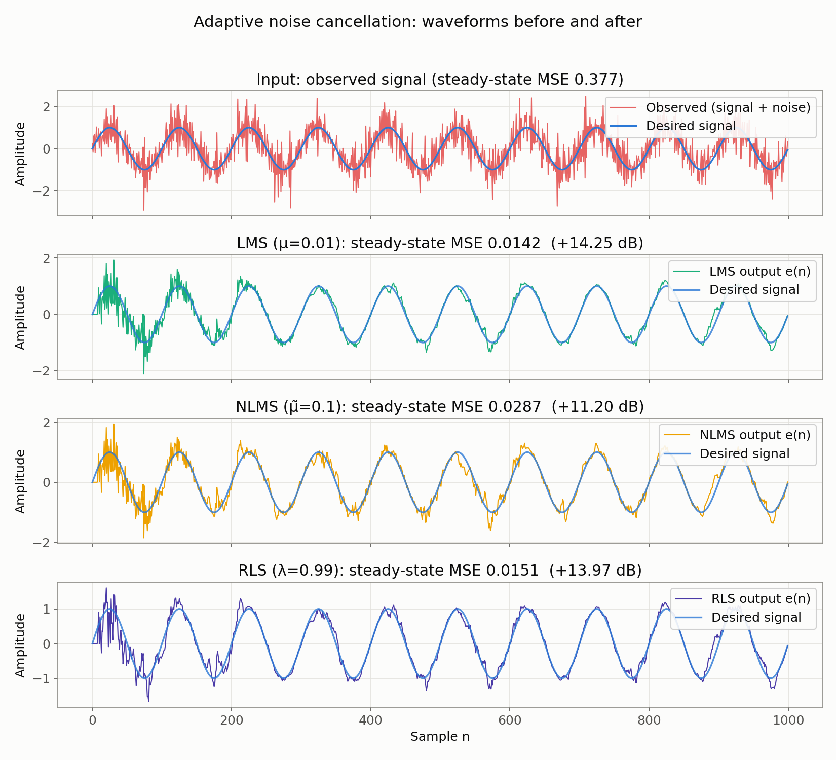
The error signal \(e(n)\) corresponds to the noise-removed signal. Looking at rows 2-4, LMS and RLS both nearly reproduce the sinusoidal desired signal, while NLMS visibly retains more residual amplitude fluctuation.
Learning Curve Visualization
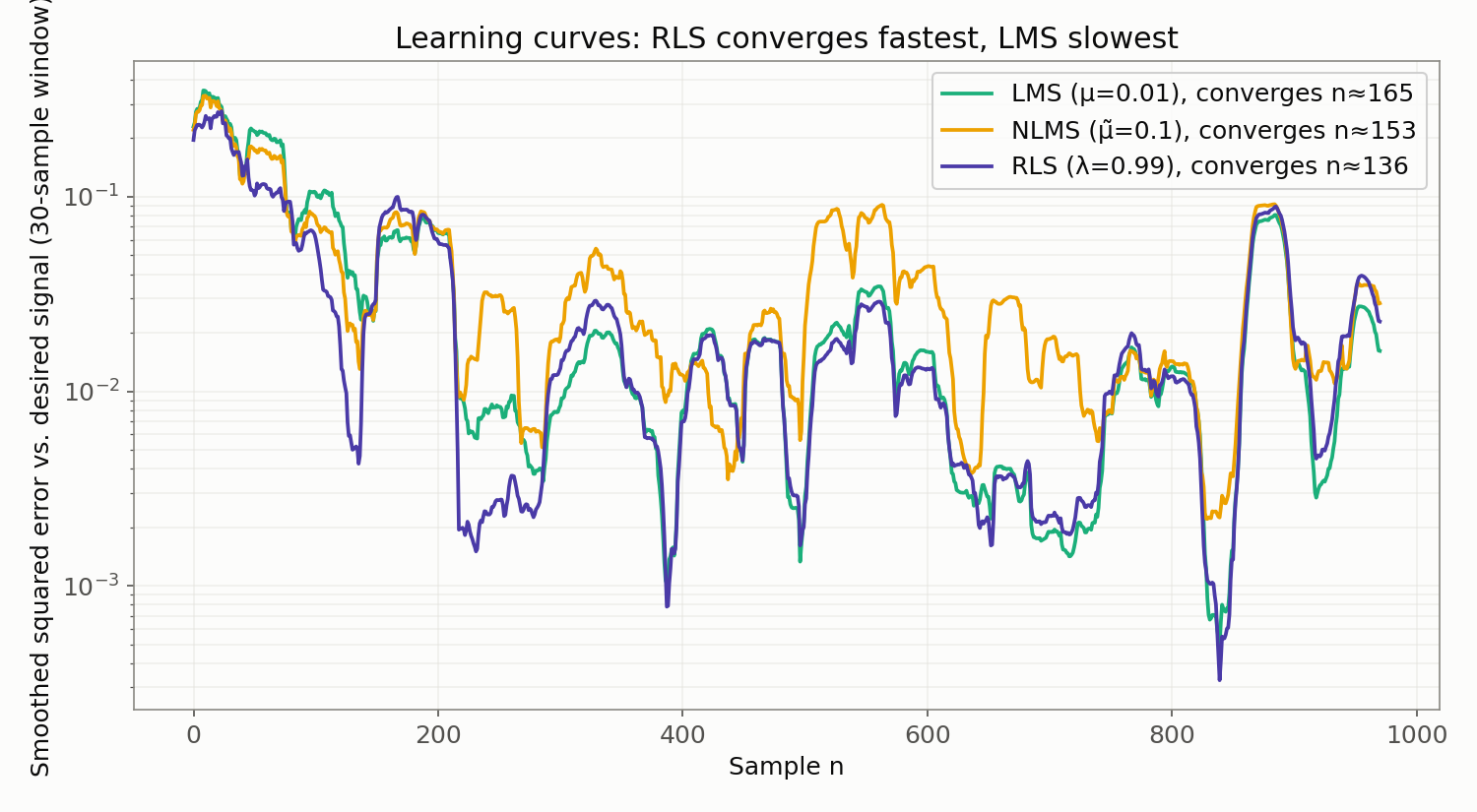
Compare convergence speeds via a learning curve (a moving average of the error relative to the desired signal).
import numpy as np

def lms_filter(x, d, M, mu):
    N = len(x)
    w = np.zeros(M)
    e = np.zeros(N)
    for n in range(M, N):
        x_vec = x[n:n-M:-1]
        e[n] = d[n] - np.dot(w, x_vec)
        w = w + mu * e[n] * x_vec
    return e

def nlms_filter(x, d, M, mu=0.5, eps=1e-8):
    N = len(x)
    w = np.zeros(M)
    e = np.zeros(N)
    for n in range(M, N):
        x_vec = x[n:n-M:-1]
        e[n] = d[n] - np.dot(w, x_vec)
        norm = np.dot(x_vec, x_vec) + eps
        w = w + (mu / norm) * e[n] * x_vec
    return e

def rls_filter(x, d, M, lam=0.99, delta=1.0):
    N = len(x)
    w = np.zeros(M)
    P = np.eye(M) / delta
    e = np.zeros(N)
    for n in range(M, N):
        x_vec = x[n:n-M:-1]
        e[n] = d[n] - np.dot(w, x_vec)
        Px = P @ x_vec
        k = Px / (lam + x_vec @ Px)
        w = w + k * e[n]
        P = (P - np.outer(k, x_vec @ P)) / lam
    return e

np.random.seed(42)
N = 1000
t = np.arange(N)
signal = np.sin(2 * np.pi * 0.01 * t)
noise_ref = np.random.randn(N)
h_true = np.array([0.5, -0.3, 0.2, -0.1])
observed = signal + np.convolve(noise_ref, h_true, mode='full')[:N]

M = 8
e_lms = lms_filter(noise_ref, observed, M, mu=0.01)
e_nlms = nlms_filter(noise_ref, observed, M, mu=0.1)
e_rls = rls_filter(noise_ref, observed, M, lam=0.99)

# Learning curve: squared deviation from the desired signal, smoothed
window = 30
def smooth_dev(e):
    return np.convolve((e - signal) ** 2, np.ones(window) / window, mode='valid')

sm_lms, sm_nlms, sm_rls = smooth_dev(e_lms), smooth_dev(e_nlms), smooth_dev(e_rls)

# Convergence point: first sample where the smoothed error drops below
# 1.5x the asymptotic error (mean of the last 200 points)
def convergence_sample(sm, factor=1.5, tail=200):
    asymptote = np.mean(sm[-tail:])
    idx = np.where(sm < asymptote * factor)[0]
    return idx[0] + window, asymptote

for name, sm in [("LMS", sm_lms), ("NLMS", sm_nlms), ("RLS", sm_rls)]:
    n_conv, asym = convergence_sample(sm)
    print(f"{name:4s}: converged at n={n_conv:4d}  (asymptotic error {asym:.5f})")
Output:
LMS : converged at n= 165  (asymptotic error 0.02036)
NLMS: converged at n= 153  (asymptotic error 0.02534)
RLS : converged at n= 136  (asymptotic error 0.02359)
The number of samples needed to first drop below 1.5x the asymptotic error (a proxy for convergence speed) was \(136\) for RLS — the fastest — followed by NLMS at \(153\) and LMS at \(165\) , the slowest. RLS is indeed fastest as theory predicts, but in this setting (\(M=8\) , white-noise input) the gap versus LMS isn’t large. LMS and NLMS Algorithms: Theory and Python Implementation shows numerically that this gap widens considerably for inputs with large eigenvalue spread (strongly autocorrelated signals).
Edge Cases and Practical Pitfalls
Three practical pitfalls that the theory and implementation above don’t reveal, each verified numerically.
1. NLMS Step Size vs. Steady-State Error Trade-off
NLMS’s convergence condition \(0 < \tilde\mu < 2\) doesn’t depend on input power, but understanding it as “anything below 2 is safe” is insufficient. The steady-state misadjustment (excess-MSE ratio) is approximately \(M \approx \tilde\mu / (2 - \tilde\mu)\) , which grows sharply as \(\tilde\mu\) increases. Let’s verify the choice of \(\tilde\mu=0.1\) used above by sweeping \(\tilde\mu\) .
import numpy as np

def nlms_filter(x, d, M, mu=0.5, eps=1e-8):
    N = len(x)
    w = np.zeros(M)
    e = np.zeros(N)
    for n in range(M, N):
        x_vec = x[n:n-M:-1]
        e[n] = d[n] - np.dot(w, x_vec)
        norm = np.dot(x_vec, x_vec) + eps
        w = w + (mu / norm) * e[n] * x_vec
    return e

np.random.seed(42)
N = 1000
t = np.arange(N)
signal = np.sin(2 * np.pi * 0.01 * t)
noise_ref = np.random.randn(N)
h_true = np.array([0.5, -0.3, 0.2, -0.1])
observed = signal + np.convolve(noise_ref, h_true, mode='full')[:N]

M = 8
steady = slice(500, 1000)
mse_before = np.mean((observed[steady] - signal[steady]) ** 2)

for mu_t in [0.5, 0.3, 0.1, 0.08, 0.05, 0.02]:
    e = nlms_filter(noise_ref, observed, M, mu=mu_t)
    mse = np.mean((e[steady] - signal[steady]) ** 2)
    pred_M = mu_t / (2 - mu_t)
    print(f"mu_tilde={mu_t:.2f}: MSE={mse:.5f}, improvement={10*np.log10(mse_before/mse):.2f} dB, "
          f"predicted misadjustment~{pred_M:.3f}")
Output:
mu_tilde=0.50: MSE=0.21244, improvement=2.50 dB, predicted misadjustment~0.333
mu_tilde=0.30: MSE=0.11465, improvement=5.17 dB, predicted misadjustment~0.176
mu_tilde=0.10: MSE=0.02866, improvement=11.20 dB, predicted misadjustment~0.053
mu_tilde=0.08: MSE=0.02136, improvement=12.47 dB, predicted misadjustment~0.042
mu_tilde=0.05: MSE=0.01223, improvement=14.89 dB, predicted misadjustment~0.026
mu_tilde=0.02: MSE=0.02052, improvement=12.65 dB, predicted misadjustment~0.010
Even at \(\tilde\mu=0.5\) — only a quarter of the stability limit \(\tilde\mu<2\) — the improvement is a mere \(2.50\) dB. Lowering \(\tilde\mu\) to \(0.05\) brings the improvement up to \(14.89\) dB, matching LMS and RLS. However \(\tilde\mu=0.02\) is actually worse (over the finite \(N=1000\) -sample window, convergence speed lags too much for the low steady-state error to help), so in practice you must tune for both convergence speed and steady-state error simultaneously. Satisfying the stability condition and achieving good performance are separate concerns.
2. Choosing the Filter Order M
Underestimating the unknown system’s order leaves bias — the coefficients can’t fully represent the true system — while overestimating it adds unnecessary degrees of freedom that increase steady-state error (misadjustment). With the true order at \(4\)
(the length of h_true), we sweep LMS’s filter order \(M\)
.
import numpy as np

def lms_filter(x, d, M, mu):
    N = len(x)
    w = np.zeros(M)
    e = np.zeros(N)
    for n in range(M, N):
        x_vec = x[n:n-M:-1]
        e[n] = d[n] - np.dot(w, x_vec)
        w = w + mu * e[n] * x_vec
    return e

np.random.seed(42)
N = 1000
t = np.arange(N)
signal = np.sin(2 * np.pi * 0.01 * t)
noise_ref = np.random.randn(N)
h_true = np.array([0.5, -0.3, 0.2, -0.1])  # true order is 4
observed = signal + np.convolve(noise_ref, h_true, mode='full')[:N]
steady = slice(500, 1000)
mse_before = np.mean((observed[steady] - signal[steady]) ** 2)

for M in [2, 4, 8, 16, 32]:
    mu = 0.01 if M <= 8 else 0.01 * 8 / M  # scale mu down to keep tr(R) comparable
    e = lms_filter(noise_ref, observed, M, mu=mu)
    mse = np.mean((e[steady] - signal[steady]) ** 2)
    print(f"M={M:>3d} (mu={mu:.4f}): MSE={mse:.5f}  ({10*np.log10(mse_before/mse):.2f} dB improvement)")
Output:
M=  2 (mu=0.0100): MSE=0.05377  (8.46 dB improvement)
M=  4 (mu=0.0100): MSE=0.00891  (16.27 dB improvement)
M=  8 (mu=0.0100): MSE=0.01420  (14.25 dB improvement)
M= 16 (mu=0.0050): MSE=0.01166  (15.10 dB improvement)
M= 32 (mu=0.0025): MSE=0.04388  (9.35 dB improvement)
\(M=4\) , matching the true order, performs best (\(16.27\) dB improvement). The undersized \(M=2\) cannot represent the unknown system and degrades to \(8.46\) dB. Increasing \(M\) to \(8\) and \(16\) — even while shrinking \(\mu\) to compensate for the growth in \(\mathrm{tr}(\mathbf{R})\) — slightly hurts performance, and \(M=32\) degrades to \(9.35\) dB. More unnecessary degrees of freedom mean more instantaneous-gradient noise (misadjustment) that can’t be suppressed. In practice, a larger filter order is not automatically safer — estimate the target system’s impulse-response length (e.g., the reverberation time of an echo path) and choose an order matched to it.
3. Correlation Between the Reference and the Desired Signal (Accidental Signal Cancellation)
Noise cancellation only works correctly under the assumption that the reference signal \(x(n)\) correlates only with the noise component and is uncorrelated with the desired signal. If this assumption breaks — the desired signal leaks into the reference (e.g., microphone bleed) — the adaptive filter mistakes the desired signal itself for removable noise and unintentionally attenuates it.
import numpy as np

def lms_filter(x, d, M, mu):
    N = len(x)
    w = np.zeros(M)
    e = np.zeros(N)
    for n in range(M, N):
        x_vec = x[n:n-M:-1]
        e[n] = d[n] - np.dot(w, x_vec)
        w = w + mu * e[n] * x_vec
    return e

np.random.seed(42)
N = 1000
t = np.arange(N)
signal = np.sin(2 * np.pi * 0.01 * t)
noise_ref = np.random.randn(N)
h_true = np.array([0.5, -0.3, 0.2, -0.1])
steady = slice(500, 1000)
M = 8

for leak in [0.0, 0.1, 0.3, 0.5, 1.0, 2.0]:
    noise_ref_leak = noise_ref + leak * signal  # desired-signal leakage into the reference
    observed_leak = signal + np.convolve(noise_ref_leak, h_true, mode='full')[:N]
    e = lms_filter(noise_ref_leak, observed_leak, M, mu=0.01)
    amp_ratio = np.std(e[steady]) / np.std(signal[steady])
    print(f"leak={leak:.2f}: output/desired amplitude ratio={amp_ratio:.4f}  "
          f"({20*np.log10(amp_ratio):+.2f} dB)")
Output:
leak=0.00: output/desired amplitude ratio=1.0291  (+0.25 dB)
leak=0.10: output/desired amplitude ratio=1.0333  (+0.28 dB)
leak=0.30: output/desired amplitude ratio=0.9321  (-0.61 dB)
leak=0.50: output/desired amplitude ratio=0.7755  (-2.21 dB)
leak=1.00: output/desired amplitude ratio=0.4900  (-6.20 dB)
leak=2.00: output/desired amplitude ratio=0.2772  (-11.14 dB)
With no leakage (the ideal condition), the output amplitude matches the desired signal almost exactly (\(+0.25\) dB). Increasing the leakage coefficient to \(1.0\) shrinks the output to \(49\%\) of the original amplitude, and at \(2.0\) it drops to \(28\%\) . The adaptive filter is cancelling part of the desired signal along with the “removable correlated component” — a failure mode that’s the mirror image of feedback howling, and just as serious in practice. (ANC headphones and echo cancellers avoid this via physical separation between the reference microphone and the desired source, or by pausing adaptation during double-talk detection.)
Recent Research: Where Adaptive Filters Fit in Hybrid AEC
Traditional adaptive filters (NLMS and Kalman-filter-family methods) remain a foundational building block of acoustic echo cancellation (AEC) research even past 2023. The ICASSP 2023 Acoustic Echo Cancellation Challenge, organized by Microsoft Research (Cutler et al., 2023, arXiv:2309.12553), is the fourth iteration of the challenge; it released both real recordings from over 10,000 devices and speakers plus synthetic data, and introduced a personalized-AEC track, a reduced 20ms latency budget, and a full-band AECMOS evaluation metric — conditions much closer to production deployment. Reports from this line of work describe a hybrid architecture as one of the leading approaches: a traditional signal-processing adaptive filter first removes the bulk of the linear echo component, and a second-stage neural network then progressively suppresses nonlinear distortion and residual echo in what remains (hybrid signal processing + deep echo cancellation). The lightweight linear adaptive filters covered in this article — NLMS and RLS — retain real practical value as that first stage: low computational cost with an explicit, provable convergence condition for the linear component. Because specific techniques and performance numbers are updated yearly, consult the latest primary sources (the challenge’s official papers and leaderboards) for current details.
Related Articles
- The RLS Algorithm in Python: Recursive Least Squares and Its Equivalence to the Kalman Filter - A follow-up that derives RLS from the matrix inversion lemma and numerically demonstrates its equivalence to the Kalman filter.
- Adaptive Filter Theory and Applications in Digital Signal Processing - Derives the Wiener-Hopf equation and steepest descent from FIR/IIR filter fundamentals — the theoretical starting point for this article.
- Exponential Moving Average (EMA) Filter Frequency Response - A representative fixed-parameter filter. Understanding EMA helps contrast with adaptive approaches.
- Wiener Filter: Theory and Python Implementation - The theoretical foundation for adaptive filters, particularly LMS.
- Kalman Filter: Theory and Python Implementation - A sequential estimation algorithm closely related to RLS.
- FIR and IIR Filter Comparison - Most adaptive filters use FIR structure. Explains the characteristics of FIR vs IIR.
- Fundamentals of Filtering in Signal Processing - A systematic overview of Kalman filter, EKF, UKF, and particle filter.
- SGD and Adam: Theory and Comparison - Optimization algorithms in deep learning based on the same stochastic gradient descent framework as LMS.
- Moving Average Filter Types and Comparison - Representative fixed filters to contrast with adaptive filters.
- Low-Pass Filter Design and Comparison - Compares frequency responses of various low-pass filters.
- Unscented Kalman Filter (UKF): Theory and Python Implementation - A nonlinear extension of the Kalman filter, which can be seen as an extension of RLS.
- LMS and NLMS Adaptive Algorithms: Theory and Python Implementation - A companion article focused on the mathematical derivation of LMS/NLMS — convergence to the Wiener solution, steady-state misadjustment, and step-size sensitivity.
- Filter Design Selection Guide: 3 axes and characteristic comparison — Use this hub to position adaptive filters against fixed alternatives during selection.
References
- Haykin, S. (2014). Adaptive Filter Theory (5th ed.). Pearson.
- Widrow, B., & Stearns, S. D. (1985). Adaptive Signal Processing. Prentice-Hall.
- Sayed, A. H. (2008). Adaptive Filters. Wiley-IEEE Press.
- Cutler, R., Saabas, A., Parnamaa, T., Purin, M., Indenbom, E., Ristea, N.-C., Guzvin, J., Gamper, H., Braun, S., & Aichner, R. (2023). ICASSP 2023 Acoustic Echo Cancellation Challenge. arXiv:2309.12553. https://arxiv.org/abs/2309.12553