What Is the Savitzky-Golay Filter?
The Savitzky-Golay filter performs local polynomial least-squares fitting within a moving window and uses the polynomial value as the smoothed result. It was proposed by Abraham Savitzky and Marcel J.E. Golay in 1964.
While moving average and EMA filters tend to blur peaks and sharp transitions, the Savitzky-Golay filter can remove noise while preserving signal features (peak positions, widths, and heights).
Key Applications
- Smoothing spectroscopic data
- Peak detection in chromatography
- Preprocessing biosignals (ECG, EEG)
- Derivative estimation of signals
Mathematical Foundation
Local Polynomial Fitting
Within a window of width \(2m+1\) (\(m\) is the number of data points on each side), a polynomial of degree \(p\) is fitted by least squares.
Setting the window center at \(n=0\) , for data points \(x_{-m}, x_{-m+1}, \dots, x_m\) , we fit:
\[ \hat{x}(n) = \sum_{k=0}^{p} a_k n^k = a_0 + a_1 n + a_2 n^2 + \cdots + a_p n^p \tag{1} \]The least squares problem minimizes the sum of squared residuals:
\[ \min_{\mathbf{a}} \sum_{n=-m}^{m} \left(x_n - \sum_{k=0}^{p} a_k n^k \right)^2 \tag{2} \]Matrix Formulation and Normal Equations
Defining the Vandermonde matrix \(\mathbf{A}\) :
\[ \mathbf{A} = \begin{bmatrix} (-m)^0 & (-m)^1 & \cdots & (-m)^p \\ (-m+1)^0 & (-m+1)^1 & \cdots & (-m+1)^p \\ \vdots & & \ddots & \vdots \\ m^0 & m^1 & \cdots & m^p \end{bmatrix} \tag{3} \]The normal equation solution is:
\[ \mathbf{a} = (\mathbf{A}^T \mathbf{A})^{-1} \mathbf{A}^T \mathbf{x} \tag{4} \]The smoothed value at the center is \(\hat{x}(0) = a_0\) , which can be expressed as a linear transformation:
\[ \hat{x}_0 = \mathbf{c}^T \mathbf{x} \tag{5} \]where \(\mathbf{c}\) is the first row of \((\mathbf{A}^T \mathbf{A})^{-1} \mathbf{A}^T\) (corresponding to \(a_0\) ). This \(\mathbf{c}\) represents the convolution coefficients of the filter.
Key Properties
- Window width \(2m+1\) vs polynomial degree \(p\) : Higher \(p\) preserves signal shape better but reduces noise removal. When \(p = 0\) , the Savitzky-Golay filter reduces to a simple moving average.
- FIR filter: The convolution coefficients \(\mathbf{c}\) depend only on window width and polynomial degree, not on the signal. It is therefore a type of FIR filter .
- Derivative estimation: Extracting \(a_1, a_2, \dots\) yields simultaneous estimates of the signal’s first and second derivatives.
Deriving the Coefficients and Their Convolution-Kernel Interpretation
Looking at the solution \(\mathbf{a} = (\mathbf{A}^T \mathbf{A})^{-1} \mathbf{A}^T \mathbf{x}\) of equation (4) as a whole matrix rather than just its first row, each row of \((\mathbf{A}^T \mathbf{A})^{-1} \mathbf{A}^T\) is a weight vector that produces one polynomial coefficient \(a_0, a_1, \dots, a_p\) as a linear combination of \(\mathbf{x}\) . Since polynomial (1) is itself a Taylor expansion, the \(k\) -th coefficient satisfies \(a_k = \hat{x}^{(k)}(0)/k!\) . The center-point estimate of the \(d\) -th derivative is therefore (with \([\cdot]_{d,:}\) denoting the \(d\) -th row of the matrix, 0-indexed):
\[ \hat{x}^{(d)}(0) = d! \cdot a_d = d! \cdot \big[(\mathbf{A}^T \mathbf{A})^{-1} \mathbf{A}^T\big]_{d,:} \, \mathbf{x} \tag{6} \]The \(d=0\) row gives the smoothing coefficients (\(\mathbf{c}\) in equation 5), \(d=1\) the first-derivative coefficients, and \(d=2\) the second-derivative coefficients. Because this coefficient vector depends only on the window width and polynomial degree, never on the signal, the Savitzky-Golay filter is an LTI (linear time-invariant) system that convolves the same coefficient vector as the window slides — exactly the same framework as any ordinary FIR filter.
Hand Calculation: window=5, p=2
As a concrete example, take \(m=2\) (window width 5) and \(p=2\) . The Vandermonde matrix from equation (3) is the following \(5 \times 3\) matrix:
\[ \mathbf{A} = \begin{bmatrix} 1 & -2 & 4 \\ 1 & -1 & 1 \\ 1 & 0 & 0 \\ 1 & 1 & 1 \\ 1 & 2 & 4 \end{bmatrix} \]Substituting into equation (4) and extracting the \(d=0\) row gives coefficients \(\left(-\frac{3}{35}, \frac{12}{35}, \frac{17}{35}, \frac{12}{35}, -\frac{3}{35}\right)\) — the well-known 5-point quadratic smoothing coefficients published in the original Savitzky & Golay (1964) paper.
Numerical Verification via Python
We implement the derivation above directly in code and compare it against scipy.signal.savgol_coeffs to confirm correctness.
import numpy as np
from math import factorial
from scipy.signal import savgol_coeffs

def sg_coeffs_manual(window_length, polyorder, deriv=0, delta=1.0):
    m = (window_length - 1) // 2
    n = np.arange(-m, m + 1)
    # Vandermonde matrix: A[i, k] = n_i^k  (same definition as eq. 3)
    A = np.vander(n, N=polyorder + 1, increasing=True)
    # Normal-equation solution matrix (A^T A)^{-1} A^T  (eq. 4)
    AtA_inv_At = np.linalg.inv(A.T @ A) @ A.T
    # d-th derivative coefficients: the d-th row scaled by d!  (eq. 6)
    row = AtA_inv_At[deriv, :]
    coeffs = factorial(deriv) * row / (delta ** deriv)
    return coeffs

# window=5, p=2 smoothing coefficients (compare with the hand calculation)
c_5_2 = sg_coeffs_manual(5, 2, deriv=0)
print("window=5, p=2:", np.round(c_5_2, 6))
# Compare against use='dot' rather than scipy's default use='conv'
# (the reason is explained after the results below)
c_scipy_dot = savgol_coeffs(5, 2, deriv=0, use='dot')
print("scipy (use=dot):", np.round(c_scipy_dot, 6))

# Exhaustive comparison across window/order/deriv combinations
cases = [(5,2,0), (7,2,0), (9,3,0), (11,3,0), (11,4,0),
         (7,2,1), (9,3,1), (11,4,1),
         (9,4,2), (11,5,2)]
max_diff = 0.0
for w, p, d in cases:
    manual = sg_coeffs_manual(w, p, deriv=d)
    scipy_dot = savgol_coeffs(w, p, deriv=d, use='dot')
    max_diff = max(max_diff, np.max(np.abs(manual - scipy_dot)))
print("Max diff across all cases (use='dot'):", max_diff)

# Also try the default setting (use='conv')
max_diff_conv = 0.0
for w, p, d in cases:
    manual = sg_coeffs_manual(w, p, deriv=d)
    scipy_conv = savgol_coeffs(w, p, deriv=d)  # default use='conv'
    max_diff_conv = max(max_diff_conv, np.max(np.abs(manual - scipy_conv)))
print("Max diff across all cases (default use='conv'):", max_diff_conv)
The results are:
window=5, p=2: both the hand calculation and the code give[-0.085714, 0.342857, 0.485714, 0.342857, -0.085714](i.e. \((-3, 12, 17, 12, -3)/35\) ) — an exact match- Max diff across all cases with
use='dot':1.965e-14(matches to floating-point precision, confirming the derivation) - Max diff against the default
use='conv':0.3249(does not match)
A practical pitfall: savgol_coeffs’s default use='conv' returns coefficients in the order expected by np.convolve — the reverse of the use='dot' array. Smoothing coefficients (\(d=0\)
) and second-derivative coefficients (\(d=2\)
) are symmetric about the window center, so reversing them changes nothing. First-derivative coefficients (\(d=1\)
), however, are antisymmetric (they flip sign), so reversing the array produces a genuinely different, sign-flipped result. Indeed, the comparison above showed mismatches of roughly 0.21–0.33 for the \(d=1\)
cases. If you derive coefficients yourself for use with np.dot, use the use='dot' convention; if you plan to feed them into np.convolve, use the use='conv' convention (reverse with [::-1]). Missing this distinction is an easy way to introduce a silent sign-flip bug in a first-derivative estimate.
Frequency Response
The frequency response of the Savitzky-Golay filter is the DTFT of the convolution coefficients \(\mathbf{c}\) :
\[ H(e^{j\omega}) = \sum_{n=-m}^{m} c_n e^{-j\omega n} \tag{7} \]Comparison with EMA and Moving Average
| Filter | Passband | Stopband | Shape Preservation | Group Delay |
|---|---|---|---|---|
| Savitzky-Golay | Wide | Gentle | Excellent | Constant (linear phase) |
| EMA | Parameter-dependent | Gentle | Moderate | Frequency-dependent |
| Moving Average | Width-dependent | Gentle | Poor | Constant (linear phase) |
| Butterworth | Sharp (order-dependent) | Sharp | Design-dependent | Nonlinear |
The Savitzky-Golay filter has linear phase response, so peak positions do not shift. This is a key difference from EMA (nonlinear phase).
Why Higher-Order Polynomial Fitting Preserves Peak Shape
The simple moving average corresponds to \(p=0\) (constant) polynomial fitting. Approximating the signal within the window by a Taylor expansion, \(x(n) = x(0) + x'(0) n + \frac{1}{2}x''(0) n^2 + \cdots\) , the expected value of the constant fit (i.e., the simple average) is:
\[ E[\bar{x}] \approx x(0) + \frac{x''(0)}{2} \cdot \frac{1}{2m+1}\sum_{n=-m}^{m} n^2 = x(0) + \frac{x''(0)}{2} \cdot \frac{m(m+1)}{3} \tag{8} \](The odd-order term \(x'(0) n\) vanishes because it sums to zero over a symmetric window.) At the top of a peak the curvature \(x''(0) < 0\) , and its coefficient \(m(m+1)/3\) grows on the order of the window width squared, so the wider the window and the sharper the signal’s curvature, the more a simple moving average systematically underestimates (blunts) the peak. EMA, despite its exponential weighting, is fundamentally the same constant approximation and carries the same bias.
Polynomial fitting with \(p \geq 2\) , by contrast, explicitly models the \(x''(0)\) term, so as long as the signal within the window is well-approximated locally by a polynomial, this bias is cancelled (up to the residual of the approximation). This is the essential difference between the Savitzky-Golay filter and the moving average or EMA; we confirm this effect quantitatively in the next section.
Python Implementation
scipy.signal.savgol_filter
With scipy.signal’s savgol_filter, you can apply the filter in a single line.
import numpy as np
from scipy.signal import savgol_filter
import matplotlib.pyplot as plt

# Generate test data
np.random.seed(42)
t = np.linspace(0, 1, 500)
# Signal with a peak + noise
signal_clean = np.sin(2 * np.pi * 3 * t) + 0.5 * np.exp(-((t - 0.3) / 0.02)**2)
noise = 0.2 * np.random.randn(len(t))
signal_noisy = signal_clean + noise

# Apply Savitzky-Golay filter
# window_length: window width (odd), polyorder: polynomial degree
y_sg = savgol_filter(signal_noisy, window_length=21, polyorder=3)

# Compare with moving average
kernel = np.ones(21) / 21
y_ma = np.convolve(signal_noisy, kernel, mode='same')

# Plot
fig, axes = plt.subplots(2, 1, figsize=(12, 8))

axes[0].plot(t, signal_clean, 'g', label='Original', linewidth=2)
axes[0].plot(t, signal_noisy, 'gray', alpha=0.5, label='Noisy')
axes[0].plot(t, y_sg, 'b', label='Savitzky-Golay (w=21, p=3)')
axes[0].plot(t, y_ma, 'r--', label='Moving Average (w=21)')
axes[0].set_title('Smoothing Comparison')
axes[0].legend()
axes[0].grid(True)

# Zoom in on peak region
mask = (t > 0.2) & (t < 0.4)
axes[1].plot(t[mask], signal_clean[mask], 'g', label='Original', linewidth=2)
axes[1].plot(t[mask], y_sg[mask], 'b', label='Savitzky-Golay')
axes[1].plot(t[mask], y_ma[mask], 'r--', label='Moving Average')
axes[1].set_title('Peak Region (Zoomed)')
axes[1].legend()
axes[1].grid(True)

plt.tight_layout()
plt.show()
Zooming into the peak region reveals that while the moving average significantly blunts the peak, the Savitzky-Golay filter preserves both peak position and height.
Comparing Boundary Handling and Padding Methods
Near the boundaries — where half the window (the \(m\)
points) extends beyond the available signal — the choice of how to treat the missing samples affects estimation accuracy. scipy.signal.savgol_filter’s mode argument offers four representative strategies:
mirror: pad by reflecting the signal (the edge sample itself is not repeated)nearest/constant: repeat the edge value (or a specified constant) outwardwrap: treat the signal as periodic and pad with values from the opposite endinterp(default): use only the \(2m+1\) boundary points and re-fit a one-sided polynomial (polynomial extrapolation) with the center shifted, at each boundary point
mirror implicitly assumes “zero derivative at the boundary” (even symmetry), constant/nearest assumes “the signal is flat at the boundary,” and wrap assumes “the signal is periodic.” Whenever the actual signal violates one of these assumptions, bias results. interp, by contrast, re-fits an actual polynomial to nearby real data using a shifted window, so it assumes neither symmetry nor periodicity — at the cost of higher variance (worse noise immunity), since the fit point sits at the edge of the window rather than the center.
To quantify this, we compare the errors of each mode on a clearly non-periodic signal with nonzero slope and curvature at both boundaries.
import numpy as np
from scipy.signal import savgol_filter

t = np.linspace(0, 1, 500)
# Non-periodic, non-flat signal (nonzero slope/curvature even at the boundaries)
signal_clean = t**2 + 0.3 * np.sin(2 * np.pi * 5 * t)

window_length = 21
polyorder = 3
m = window_length // 2  # 10

modes = ['mirror', 'nearest', 'constant', 'wrap', 'interp']
n_trials = 200
noise_sigma = 0.15

boundary_rmse = {mode: [] for mode in modes}
interior_rmse = {mode: [] for mode in modes}

rng = np.random.default_rng(7)
for _ in range(n_trials):
    noise = noise_sigma * rng.standard_normal(len(t))
    signal_noisy = signal_clean + noise
    for mode in modes:
        y = savgol_filter(signal_noisy, window_length, polyorder, mode=mode)
        err_boundary = np.concatenate([y[:m] - signal_clean[:m], y[-m:] - signal_clean[-m:]])
        err_interior = y[m:-m] - signal_clean[m:-m]
        boundary_rmse[mode].append(np.sqrt(np.mean(err_boundary**2)))
        interior_rmse[mode].append(np.sqrt(np.mean(err_interior**2)))

print(f"{'mode':>10} {'boundary RMSE':>15} {'interior RMSE':>15}")
for mode in modes:
    print(f"{mode:>10} {np.mean(boundary_rmse[mode]):15.5f} {np.mean(interior_rmse[mode]):15.5f}")

# Decompose bias and variance at the very first sample (t=0, true value=0)
first_vals = {mode: [] for mode in modes}
rng = np.random.default_rng(7)
for _ in range(n_trials):
    noise = noise_sigma * rng.standard_normal(len(t))
    signal_noisy = signal_clean + noise
    for mode in modes:
        y = savgol_filter(signal_noisy, window_length, polyorder, mode=mode)
        first_vals[mode].append(y[0])
print(f"\ntrue value at t=0: {signal_clean[0]:.5f}")
for mode in modes:
    vals = np.array(first_vals[mode])
    print(f"{mode:>10}: bias={np.mean(vals) - signal_clean[0]:+.5f}  std={np.std(vals):.5f}")
The results (averaged over 200 trials, window=21, polyorder=3, noise \(\sigma=0.15\) ) are:
| mode | Boundary RMSE | Interior RMSE (reference) |
|---|---|---|
mirror | 0.05674 | 0.04926 |
nearest | 0.05880 | 0.04926 |
constant | 0.15530 | 0.04926 |
wrap | 0.21441 | 0.04926 |
interp | 0.06485 | 0.04926 |
The interior RMSE is identical across all modes (boundary handling only affects the edge samples), but the boundary RMSE differs sharply. wrap degrades badly (0.214, more than 4x the interior value) because this signal is not periodic, and constant also degrades to more than 3x the interior value because of its incorrect flat-boundary assumption.
Looking only at the very first sample (\(t=0\) , true value 0) reveals the bias-variance trade-off clearly.
| mode | Bias | Std. dev. |
|---|---|---|
mirror | +0.04124 | 0.07197 |
nearest | +0.01796 | 0.09486 |
constant | +0.02033 | 0.03931 |
wrap | +0.45766 | 0.04949 |
interp | -0.00238 | 0.11948 |
interp (the default), which assumes neither symmetry, flatness, nor periodicity at the boundary, brings the bias down to essentially zero (-0.0024), but its variance is the worst of all the modes (std 0.1195, roughly 3x that of constant) because it fits a point away from the window center. wrap shows a strikingly large bias (+0.458), confirming it is unsuitable for non-periodic data like this one. In short: choose boundary handling based on which assumption about the signal’s boundary behavior actually holds. Avoid wrap unless the signal is genuinely periodic, and prefer interp (the default) or mirror when there is a clear trend at the boundary.
Parameter Effects
Visualize how window length and polynomial order affect filter characteristics.
import numpy as np
from scipy.signal import savgol_filter
import matplotlib.pyplot as plt

np.random.seed(42)
t = np.linspace(0, 1, 500)
signal_clean = np.sin(2 * np.pi * 3 * t) + 0.5 * np.exp(-((t - 0.3) / 0.02) ** 2)
signal_noisy = signal_clean + 0.2 * np.random.randn(len(t))

fig, axes = plt.subplots(1, 2, figsize=(14, 5))

# Effect of window length (fixed polyorder=3)
for w in [5, 11, 21, 41]:
    y = savgol_filter(signal_noisy, window_length=w, polyorder=3)
    axes[0].plot(t, y, label=f'w={w}')
axes[0].plot(t, signal_clean, 'k--', alpha=0.5, label='Original')
axes[0].set_title('Effect of Window Length (polyorder=3)')
axes[0].legend()
axes[0].grid(True)

# Effect of polynomial order (fixed window=21)
for p in [0, 1, 2, 3, 5]:
    y = savgol_filter(signal_noisy, window_length=21, polyorder=p)
    axes[1].plot(t, y, label=f'p={p}')
axes[1].plot(t, signal_clean, 'k--', alpha=0.5, label='Original')
axes[1].set_title('Effect of Polynomial Order (window=21)')
axes[1].legend()
axes[1].grid(True)

plt.tight_layout()
plt.show()
Qualitative observations:
- Larger window width provides stronger smoothing but may lose fine signal structure
- Polynomial order \(p = 0\) is equivalent to a simple moving average
- When \(p\) approaches the window width, noise removal becomes negligible
To back up these qualitative trends with numbers, we sweep window length and polynomial order on a grid and measure the RMSE against the true signal (evaluated only on the interior region, excluding the boundaries).
import numpy as np
from scipy.signal import savgol_filter

t = np.linspace(0, 1, 500)
signal_clean = np.sin(2 * np.pi * 3 * t) + 0.5 * np.exp(-((t - 0.3) / 0.02) ** 2)

windows = [5, 9, 11, 15, 21, 31, 41, 61]
orders = [0, 2, 3, 5]
sigma = 0.2
n_trials = 80
m_exclude = 30

results = {p: [] for p in orders}
for p in orders:
    for w in windows:
        if p >= w:
            results[p].append(None)
            continue
        rng = np.random.default_rng(hash((w, p)) % (2**31))
        errs = []
        for _ in range(n_trials):
            noise = sigma * rng.standard_normal(len(t))
            y = signal_clean + noise
            ys = savgol_filter(y, w, p)
            e = ys[m_exclude:-m_exclude] - signal_clean[m_exclude:-m_exclude]
            errs.append(np.sqrt(np.mean(e**2)))
        results[p].append(np.mean(errs))

for p in orders:
    row = ", ".join(f"w={w}:{v:.4f}" for w, v in zip(windows, results[p]) if v is not None)
    print(f"p={p}: {row}")
The results (RMSE averaged over 80 trials, noise \(\sigma=0.2\) ) are:
| window\order | p=0 | p=2 | p=3 | p=5 |
|---|---|---|---|---|
| 5 | 0.0892 | 0.1397 | 0.1386 | — |
| 9 | 0.0670 | 0.1010 | 0.1010 | 0.1291 |
| 11 | 0.0603 | 0.0912 | 0.0910 | 0.1142 |
| 15 | 0.0535 | 0.0770 | 0.0779 | 0.0972 |
| 21 | 0.0513 | 0.0656 | 0.0651 | 0.0822 |
| 31 | 0.0628 | 0.0549 | 0.0557 | 0.0674 |
| 41 | 0.0889 | 0.0498 | 0.0501 | 0.0598 |
| 61 | 0.1607 | 0.0524 | 0.0518 | 0.0521 |
Panel (a) below plots this grid.
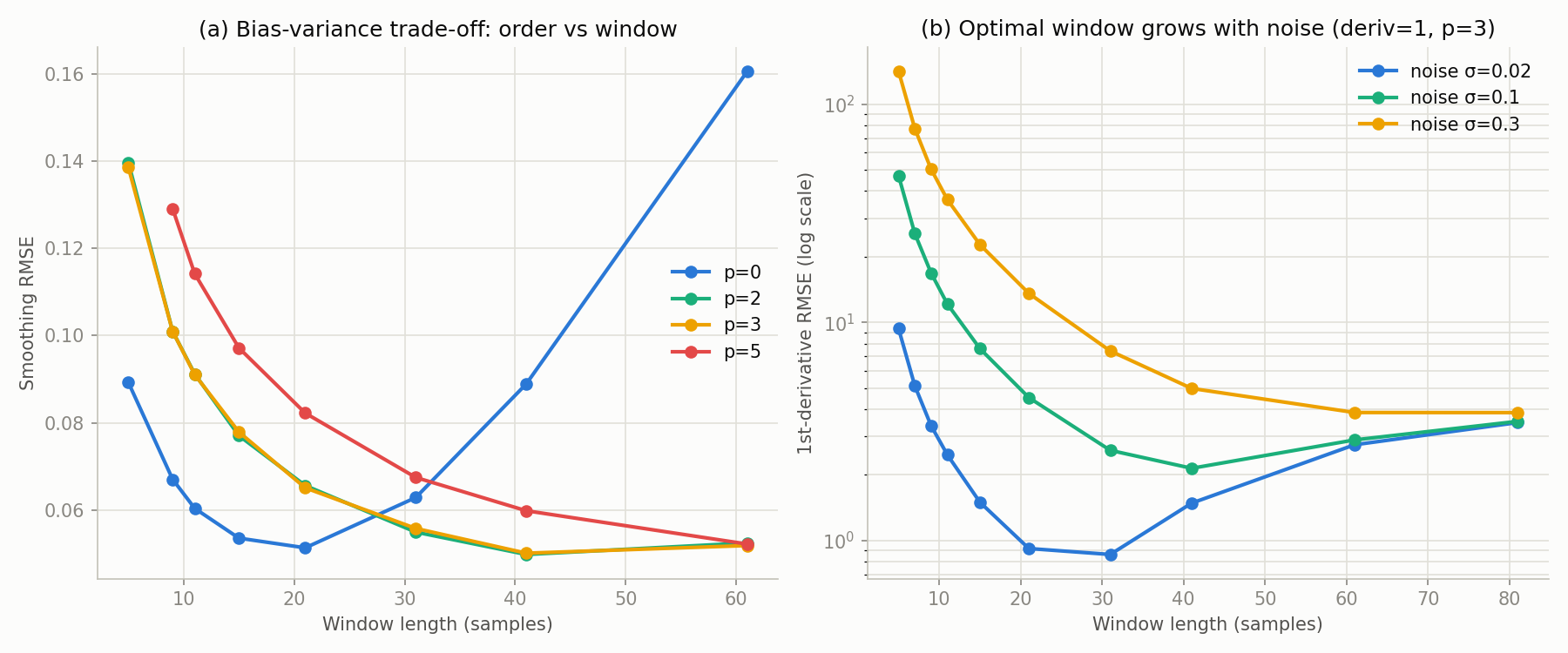
This grid reveals a trade-off structure that isn’t captured by “bigger window / higher order is always better”:
- For \(p=0\) (moving average), RMSE is minimized at \(w=21\) (0.0513) and degrades rapidly beyond that (\(w=61\) gives 0.1607, more than 3x the minimum). This is exactly the curvature bias from equation (8) growing with the square of the window width.
- For \(p=2,3\) , RMSE keeps improving monotonically up to \(w=41\) (0.0498, 0.0501). Since curvature is modeled explicitly, a wider window can average out more noise without introducing peak bias.
- \(p=5\) is worse than \(p=2,3\) at every window length (e.g., at \(w=21\) , 0.0822 vs. 0.0651-0.0656). Pushing the order too high lets the fit track the noise itself (overfitting), increasing variance and hurting performance.
In other words, we’ve measured directly the trade-off where “too high an order overfits noise, and too wide a window (with insufficient order) distorts peak shape” — confirming the conventional guidance that \(p=2\) or \(p=3\) with \(w=21\) –\(41\) works well for this signal and noise level.
Comparing Peak-Shape Preservation: Moving Average, EMA, and Savitzky-Golay
We now quantitatively confirm, in terms of actual peak-preservation performance, the reasoning derived above (equation 8) for why higher-order polynomials preserve peak shape. We add noise to an isolated Gaussian peak (amplitude 1, FWHM about 33 samples) and compare the recovered peak height after smoothing with a moving average, EMA, and Savitzky-Golay (\(p=2,3,5\) ).
import numpy as np
from scipy.signal import savgol_filter

t = np.linspace(0, 1, 500)
peak_center, peak_width, peak_height = 0.5, 0.02, 1.0
signal_clean = peak_height * np.exp(-((t - peak_center) / peak_width) ** 2)
true_peak_idx = np.argmax(signal_clean)
true_peak_val = signal_clean[true_peak_idx]

def moving_average(x, w):
    kernel = np.ones(w) / w
    return np.convolve(x, kernel, mode='same')

def ema(x, alpha):
    y = np.zeros_like(x)
    y[0] = x[0]
    for i in range(1, len(x)):
        y[i] = alpha * x[i] + (1 - alpha) * y[i - 1]
    return y

n_trials = 200
sigma = 0.1
w = 21
alpha = 2 / (w + 1)  # EMA coefficient matched to an equivalent span

methods = {
    "Moving Average": lambda y: moving_average(y, w),
    "EMA": lambda y: ema(y, alpha),
    "SG (p=2)": lambda y: savgol_filter(y, w, 2),
    "SG (p=3)": lambda y: savgol_filter(y, w, 3),
    "SG (p=5)": lambda y: savgol_filter(y, w, 5),
}

peak_heights = {name: [] for name in methods}
rng = np.random.default_rng(5)
for _ in range(n_trials):
    noise = sigma * rng.standard_normal(len(t))
    y = signal_clean + noise
    search = slice(max(0, true_peak_idx - 30), true_peak_idx + 31)
    for name, fn in methods.items():
        yf = fn(y)
        peak_heights[name].append(np.max(yf[search]))

print(f"true peak height = {true_peak_val:.3f}")
for name, vals in peak_heights.items():
    vals = np.array(vals)
    mean = np.mean(vals)
    bias_pct = (mean / true_peak_val - 1) * 100
    print(f"{name:>16}: mean peak={mean:.4f} (bias {bias_pct:+.1f}%), std={np.std(vals):.4f}")
The results (window=21-equivalent, noise \(\sigma=0.1\) , averaged over 200 trials, true peak height=0.997) are:
| Method | Mean peak height | Bias | Std. dev. |
|---|---|---|---|
| Moving Average | 0.7289 | -26.9% | 0.0195 |
| EMA | 0.6845 | -31.4% | 0.0197 |
| SG (p=2) | 0.9665 | -3.1% | 0.0305 |
| SG (p=3) | 0.9665 | -3.1% | 0.0305 |
| SG (p=5) | 1.0035 | +0.6% | 0.0393 |
Both the moving average and EMA underestimate the peak height by 27–31%, whereas Savitzky-Golay with \(p=2,3\)
keeps the bias to about 3% (at the cost of somewhat higher standard deviation). \(p=5\)
brings the bias to nearly zero but tracks noise more closely, giving the largest standard deviation. Note also that SG (p=2) and SG (p=3) agree to the last decimal digit shown — this is not a coincidence, but a numerical confirmation of the well-known fact that on a symmetric window, raising the order by one from an even \(p\)
(i.e. \(p \to p+1\)
) leaves the smoothing coefficients themselves unchanged (the \(d=0\)
row of equation 6 is identical).
We can also use f''(peak) and equation (8) to predict the moving-average bias ahead of time:
h = 1e-6
f = lambda tt: peak_height * np.exp(-((tt - peak_center) / peak_width) ** 2)
f2 = (f(peak_center + h) - 2 * f(peak_center) + f(peak_center - h)) / h**2
dt = t[1] - t[0]
f2_sample = f2 * dt**2  # convert to per-sample^2 units
m = w // 2
predicted_bias_pct = (f2_sample / 2) * (m * (m + 1) / 3) / true_peak_val * 100
print(f"predicted bias from eq. (8): {predicted_bias_pct:.1f}%  (measured: -26.9%)")
This calculation predicts a bias of about -36.9%, which is the same order of magnitude as the measured -26.9% (since eq. 8 is a second-order Taylor approximation, and the window here is not small compared to the peak width, higher-order terms mean the two don’t match exactly — but this confirms that eq. 8 correctly identifies both the qualitative and quantitative origin of the moving average’s peak bias).
Derivative Estimation Precision: The Noise-Immunity vs. Bias Trade-off
A key feature of the Savitzky-Golay filter is simultaneous smoothing and derivative estimation. From equation (6), the \(d\) -th derivative estimate is the inner product \(\hat{x}^{(d)}(0) = \mathbf{c}_d^T \mathbf{x}\) of the coefficient vector \(\mathbf{c}_d\) with the observed data \(\mathbf{x} = \mathbf{s} + \mathbf{e}\) (\(\mathbf{s}\) : true signal, \(\mathbf{e}\) : iid noise with variance \(\sigma^2\) ). Its variance therefore has a closed analytical form — the noise gain:
\[ \mathrm{Var}\big[\hat{x}^{(d)}(0)\big] = \sigma^2 \, \mathbf{c}_d^T \mathbf{c}_d = \sigma^2 \sum_{n=-m}^{m} c_{d,n}^2 \tag{9} \]We first verify this formula by applying the SG derivative filter to pure white noise and comparing the theoretical variance with the empirical variance of the output.
import numpy as np
from scipy.signal import savgol_coeffs

rng = np.random.default_rng(0)
sigma = 1.0
N = 200000
noise = sigma * rng.standard_normal(N)

cases = [(11, 2, 0), (21, 2, 0), (41, 2, 0),
         (11, 3, 1), (21, 3, 1), (41, 3, 1),
         (11, 4, 2), (21, 4, 2), (41, 4, 2)]

for w, p, d in cases:
    c = savgol_coeffs(w, p, deriv=d, use='dot')
    theory = sigma**2 * np.sum(c**2)
    filtered = np.convolve(noise, c[::-1], mode='valid')  # apply under the 'dot' convention
    emp = np.var(filtered)
    print(f"w={w:3d} p={p} d={d}: theory={theory:.6f}  empirical={emp:.6f}")
The results below show theory and empirical values agreeing to within 1%, numerically confirming equation (9).
| window | order | deriv | theory \(\sigma^2\sum c^2\) | empirical variance |
|---|---|---|---|---|
| 11 | 2 | 0 | 0.207459 | 0.206531 |
| 21 | 2 | 0 | 0.107551 | 0.107034 |
| 41 | 2 | 0 | 0.054933 | 0.054761 |
| 11 | 3 | 1 | 0.060379 | 0.060377 |
| 21 | 3 | 1 | 0.008249 | 0.008215 |
| 41 | 3 | 1 | 0.001093 | 0.001083 |
| 11 | 4 | 2 | 0.065365 | 0.065790 |
| 21 | 4 | 2 | 0.002262 | 0.002254 |
| 41 | 4 | 2 | 0.000077 | 0.000076 |
This noise gain decreases rapidly as window width \(w\) grows, and the rate of decrease is steeper for higher derivative orders. Comparing \(w=11 \to 41\) (about 3.7x) in the table above: the noise gain shrinks only about 3.8x for smoothing (\(d=0\) ), but about 55x for the first derivative (\(d=1\) ) and about 850x for the second derivative (\(d=2\) ). This means the benefit of a wider window for suppressing noise is much larger for higher derivative orders (at the cost of a correspondingly larger bias impact).
On the other hand, widening the window increases bias from higher-order signal content that the local polynomial cannot capture. We check how the optimal window shifts with noise level, using a signal with a known analytical first derivative.
import numpy as np
from scipy.signal import savgol_filter

t = np.linspace(0, 1, 500)
dt = t[1] - t[0]
signal_clean = np.sin(2 * np.pi * 3 * t) + 0.5 * np.exp(-((t - 0.3) / 0.02) ** 2)
dy_true = 2 * np.pi * 3 * np.cos(2 * np.pi * 3 * t) + \
          0.5 * (-2 * (t - 0.3) / 0.02**2) * np.exp(-((t - 0.3) / 0.02) ** 2)

windows_b = [5, 7, 9, 11, 15, 21, 31, 41, 61, 81]
noise_levels = [0.02, 0.1, 0.3]
polyorder = 3
m_exclude = 30

for sigma in noise_levels:
    rmses = []
    for w in windows_b:
        rng = np.random.default_rng(int(sigma * 1000) + w)
        errs = []
        for _ in range(60):
            noise = sigma * rng.standard_normal(len(t))
            y = signal_clean + noise
            dy = savgol_filter(y, w, polyorder, deriv=1, delta=dt)
            e = dy[m_exclude:-m_exclude] - dy_true[m_exclude:-m_exclude]
            errs.append(np.sqrt(np.mean(e**2)))
        rmses.append(np.mean(errs))
    best_idx = int(np.argmin(rmses))
    print(f"sigma={sigma}: best window={windows_b[best_idx]}, RMSE={rmses[best_idx]:.4f}")
The results (first derivative, polyorder=3, interior-only RMSE, averaged over 60 trials) are shown below; panel (b) of the figure above plots this RMSE curve.
| Noise \(\sigma\) | Best window | Min RMSE |
|---|---|---|
| 0.02 | 31 | 0.8641 |
| 0.1 | 41 | 2.1455 |
| 0.3 | 61-81 (nearly flat) | 3.8606 |
At low noise (\(\sigma=0.02\) ), a narrower window (31) is optimal, but as noise increases the optimal window grows monotonically (41 → 61-81), and at \(\sigma=0.3\) there is essentially no further improvement past window 61. This directly demonstrates that the point where the noise-gain reduction from equation (9) balances the bias increase from a wider window shifts with the noise level. The practical takeaway is that derivative estimation under noisier observations requires an even larger window than ordinary smoothing does.
Frequency Response Visualization
import numpy as np
import matplotlib.pyplot as plt
from scipy.signal import savgol_coeffs, freqz

# Get filter coefficients
for w, p in [(11, 2), (21, 3), (41, 3)]:
    coeffs = savgol_coeffs(w, p)
    freq, response = freqz(coeffs, worN=2048)
    plt.plot(freq / np.pi, 20 * np.log10(np.abs(response)),
             label=f'w={w}, p={p}')

plt.xlabel('Normalized Frequency (×π rad/sample)')
plt.ylabel('Gain (dB)')
plt.title('Savitzky-Golay Filter Frequency Response')
plt.legend()
plt.grid(True)
plt.ylim(-60, 5)
plt.tight_layout()
plt.show()
Choosing the Right Filter
| Use Case | Recommended Filter | Reason |
|---|---|---|
| Smoothing while preserving peaks | Savitzky-Golay | Polynomial fitting preserves shape |
| Real-time smoothing | EMA | \(O(1)\) computation, causal |
| Removing specific frequency bands | Butterworth / Notch | Sharp cutoff characteristics |
| Known noise statistics | Wiener / Kalman | Statistically optimal |
| Derivative estimation | Savitzky-Golay | Integrated smoothing and differentiation |
| Non-stationary signals | Wavelet | Time-frequency analysis |
Recent Research Trends
Although the Savitzky-Golay filter is over 60 years old, research continues past 2023 to address the challenge that fixed window width and polynomial order cannot be optimal across an entire signal (as we measured directly in the “Window Length and Polynomial Order Selection Guide” section above).
- Adaptive windowing for spectral analysis: Altynbekov et al. (2023) proposed a sliding-window variant of the Savitzky-Golay filter for denoising terahertz absorption spectra, varying the window rather than fixing it across the whole spectrum. Separately, an adaptive filter that combines a standard Savitzky-Golay filter with independent component analysis (ICA) has been proposed for gas-mixture absorption spectra; on experimental SO2/H2O gas-mixture data, the relative error in retrieved concentration was reported to be about 3.7x smaller than with a standard fixed-parameter Savitzky-Golay filter (published in Atmospheric and Oceanic Optics). Both efforts share the same motivation as the bias-variance trade-off derived in this article: strong and weak absorption lines require different optimal smoothing parameters.
- Comparison with deep learning on Raman spectroscopy data: Gil et al. (2023, Journal of Raman Spectroscopy) benchmarked a single-layer convolutional neural network trained on simulated data against Savitzky-Golay filtering for denoising Raman spectra. At low signal-to-noise ratios, the convolutional network was reported to outperform Savitzky-Golay filtering; nonetheless, Savitzky-Golay remains one of the most widely used preprocessing methods in Raman spectroscopy, owing to its low computational cost and interpretability.
Taken together, these trends show that the underlying mathematics of the Savitzky-Golay filter — the least-squares polynomial fitting derived in this article — hasn’t changed, but research is progressing along two complementary tracks: dynamically adapting window width and order to the data, and benchmarking against deep-learning-based alternatives. Note that these are application-specific results, not evidence of a universally adopted successor algorithm.
Related Articles
- Exponential Moving Average (EMA) Filter Frequency Response - EMA is a first-order IIR filter with low computational cost, but lacks the shape preservation capability of Savitzky-Golay.
- Moving Average Filter Types and Comparison - Setting the Savitzky-Golay polynomial order to 0 yields a simple moving average.
- FFT: Algorithm and Python Implementation - The foundational algorithm for analyzing filter frequency characteristics.
- Low-Pass Filter Design and Comparison - Compares frequency response and group delay of various low-pass filters.
- FIR and IIR Filter Comparison - The Savitzky-Golay filter is a type of FIR filter with linear phase characteristics.
- Butterworth Filter Design and Python Implementation - An IIR filter for cases requiring sharper cutoff characteristics.
- Wiener Filter: Theory and Python Implementation - Statistically optimal filter design, effective when noise statistics are known.
- Window Functions and Power Spectral Density (PSD) - Window function theory related to Savitzky-Golay window width selection.
- Matplotlib Tips: Creating Publication-Quality Plots - Tips for creating high-quality plots of frequency responses and smoothing results.
- Notch Filter Design and Python Implementation - A filter for removing specific frequencies, a different approach from Savitzky-Golay.
- Kalman Filter: Theory and Python Implementation - Probabilistic filtering based on state-space models, a fundamentally different paradigm from Savitzky-Golay.
- Filter Design Selection Guide: 3 axes and characteristic comparison — Use this hub to position the Savitzky-Golay filter against alternatives during selection.
References
- Savitzky, A., & Golay, M. J. E. (1964). Smoothing and Differentiation of Data by Simplified Least Squares Procedures. Analytical Chemistry, 36(8), 1627-1639.
- Schafer, R. W. (2011). What Is a Savitzky-Golay Filter? IEEE Signal Processing Magazine, 28(4), 111-117.
- Altynbekov, A., et al. (2023). The possibility of increasing the efficiency of terahertz absorption spectra noise reduction using a sliding window variant of Savitzky-Golay filter.
- Gil, D., et al. (2023). Denoising Raman spectra using a single layer convolutional model trained on simulated data. Journal of Raman Spectroscopy.
- Adaptive Savitzky–Golay Filter for Denoising Gas Mixture Absorption Spectra. Atmospheric and Oceanic Optics.
- scipy.signal.savgol_filter documentation